## Surface Plots: Hessian vs. Random Directions
### Overview
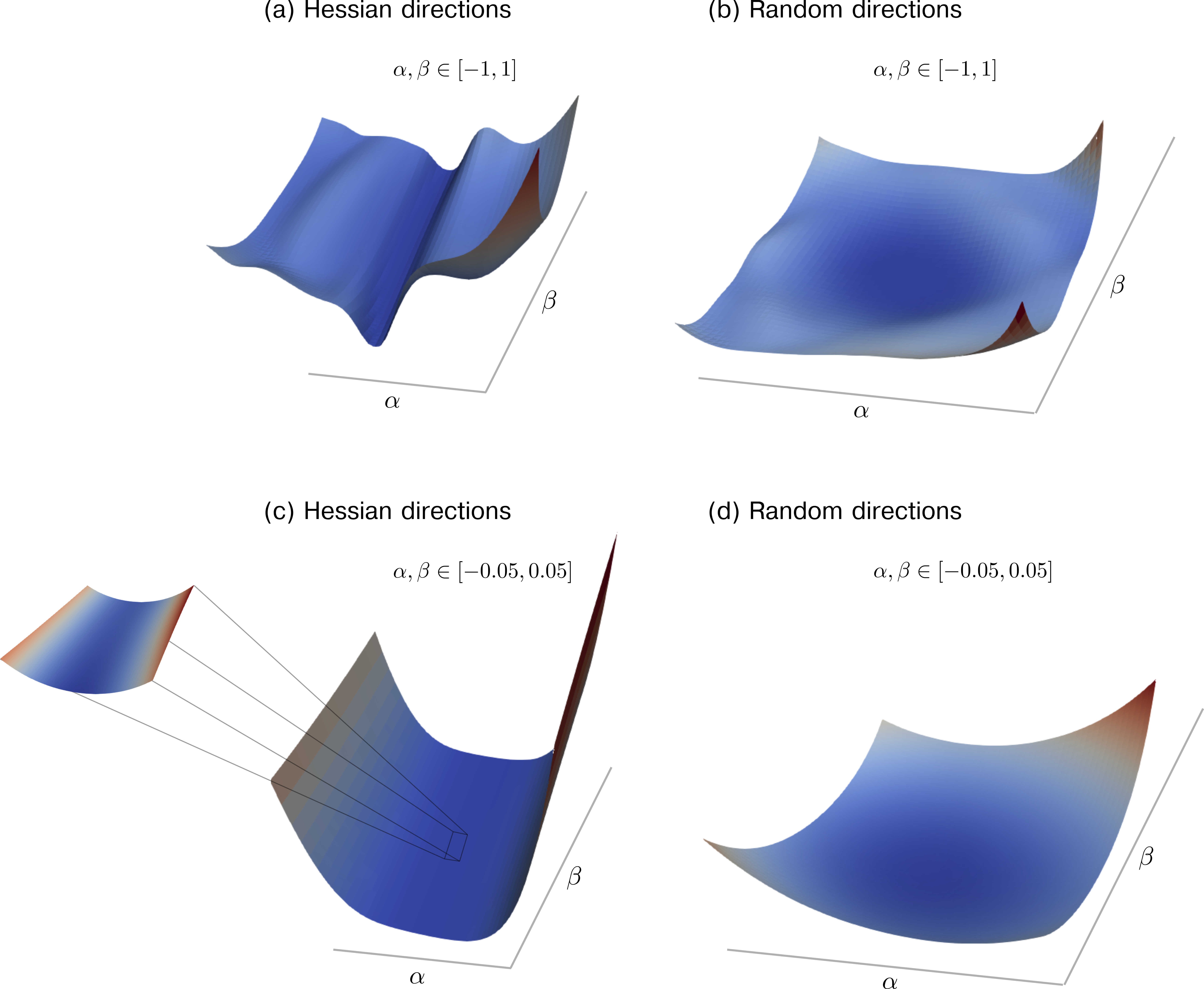
The image presents four 3D surface plots, arranged in a 2x2 grid. Each plot visualizes a function's behavior with respect to two variables, alpha (α) and beta (β). The plots are distinguished by the method used to determine the directions (Hessian vs. Random) and the range of alpha and beta values. The surface color represents the function's output, transitioning from blue (low values) to red (high values).
### Components/Axes
Each plot has the following components:
* **Axes:** Two axes labeled α (alpha) and β (beta) form the base of each plot.
* **Surface:** A colored surface represents the function's output for different combinations of α and β. The color gradient ranges from blue to red.
* **Titles:** Each plot has a title indicating the direction type (Hessian or Random) and a range for α and β.
Specific labels and ranges:
* **(a) Hessian directions:** α, β ∈ [-1, 1]
* **(b) Random directions:** α, β ∈ [-1, 1]
* **(c) Hessian directions:** α, β ∈ [-0.05, 0.05]
* **(d) Random directions:** α, β ∈ [-0.05, 0.05]
### Detailed Analysis
**Plot (a): Hessian directions, α, β ∈ [-1, 1]**
* The surface exhibits significant undulations and variations.
* There's a distinct "valley" or trough running across the surface.
* The color varies considerably, indicating a wide range of function values.
* The surface reaches higher values (red) at the edges, particularly along the β axis.
**Plot (b): Random directions, α, β ∈ [-1, 1]**
* The surface is smoother compared to plot (a).
* It has a bowl-like shape, with the lowest point in the center.
* The color gradient is more gradual, suggesting a smaller range of function values.
* The surface also reaches higher values (red) at the edges, particularly along the β axis.
**Plot (c): Hessian directions, α, β ∈ [-0.05, 0.05]**
* This plot shows a zoomed-in view of the Hessian directions around the origin.
* The surface is relatively smooth and bowl-shaped.
* The color is predominantly blue, indicating low function values in this region.
* A small inset diagram shows a further zoomed-in view of a region on the surface. The inset is connected to the main plot by several lines.
**Plot (d): Random directions, α, β ∈ [-0.05, 0.05]**
* This plot shows a zoomed-in view of the Random directions around the origin.
* The surface is smooth and bowl-shaped, similar to plot (c).
* The color is predominantly blue, indicating low function values in this region.
### Key Observations
* **Direction Type:** Hessian directions (a, c) result in more complex and variable surfaces compared to Random directions (b, d).
* **Range of α and β:** Reducing the range of α and β to [-0.05, 0.05] (c, d) reveals a smoother, bowl-shaped behavior near the origin for both Hessian and Random directions.
* **Surface Color:** The color gradient indicates the function's output value, with blue representing lower values and red representing higher values.
### Interpretation
The plots illustrate how different methods for choosing directions (Hessian vs. Random) affect the shape of the function's surface. Hessian directions, which are based on the function's curvature, lead to more complex and potentially unstable behavior, especially when considering a wider range of α and β values. Random directions, on the other hand, result in a smoother and more predictable surface.
The zoomed-in views (c, d) suggest that near the origin, both methods exhibit a similar bowl-shaped behavior, indicating a local minimum. However, the behavior diverges significantly as α and β move away from the origin, as seen in plots (a) and (b). This suggests that the choice of direction method can have a significant impact on the optimization process, particularly when dealing with non-convex functions.