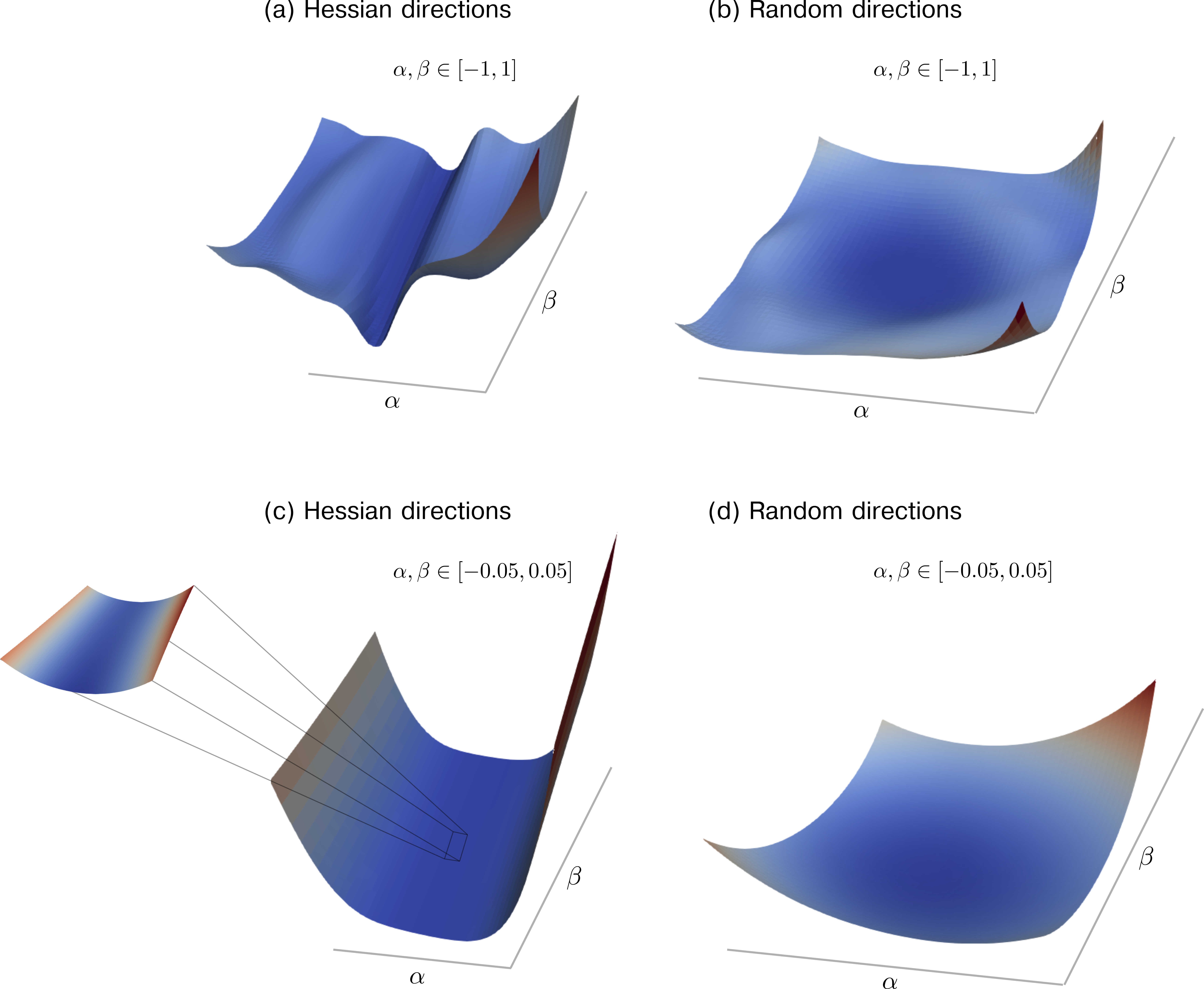
\n ## 3D Surface Plots: Comparison of Hessian vs. Random Direction Landscapes ### Overview The image displays four 3D surface plots arranged in a 2x2 grid. Each plot visualizes a mathematical function's surface over a two-dimensional parameter space defined by variables α (alpha) and β (beta). The plots are grouped into two categories: "Hessian directions" (left column) and "Random directions" (right column). The top row shows the landscape over a broad range, while the bottom row shows a zoomed-in view near the origin. The surfaces are colored with a gradient, where blue represents lower function values and red/brown represents higher values. ### Components/Axes * **Titles:** * Top-left (a): "Hessian directions" * Top-right (b): "Random directions" * Bottom-left (c): "Hessian directions" * Bottom-right (d): "Random directions" * **Axis Labels:** All four plots have identical axis labels. * Horizontal axis (front): α (alpha) * Horizontal axis (side): β (beta) * Vertical axis: Implied to be a function value, f(α, β), but not explicitly labeled. * **Range Annotations:** * Top Row (a & b): `α, β ∈ [-1, 1]` (indicating the parameters range from -1 to 1). * Bottom Row (c & d): `α, β ∈ [-0.05, 0.05]` (indicating a zoomed-in view near zero). * **Color Mapping (Implicit Legend):** The surface color corresponds to the vertical (function) value. The gradient transitions from deep blue (lowest points) through light blue/white to red/brown (highest points). ### Detailed Analysis **Plot (a) - Hessian directions, Range [-1, 1]:** * **Trend:** The surface is highly non-convex and complex. It features multiple local minima (deep blue valleys) and maxima (red/brown peaks). The landscape is "wrinkled" with significant curvature changes. * **Spatial Details:** A prominent deep blue valley runs diagonally from the front-left towards the center. Several sharp red peaks are visible, particularly one on the right side and another towards the back. The surface exhibits saddle points and ridges. **Plot (b) - Random directions, Range [-1, 1]:** * **Trend:** The surface is much smoother and simpler compared to (a). It resembles a broad, shallow basin or a slightly distorted paraboloid. * **Spatial Details:** The lowest point (deepest blue) is near the center of the α-β plane. The function value increases smoothly and monotonically as one moves away from the center towards the edges of the [-1, 1] domain, transitioning to red/brown at the corners. There are no visible local minima or complex features. **Plot (c) - Hessian directions, Range [-0.05, 0.05]:** * **Trend:** This is a zoomed-in view of the landscape near the origin (α=0, β=0) for the Hessian case. The surface shows a distinct saddle shape or a sharp valley. * **Spatial Details:** A deep blue valley runs through the center. The function increases sharply (to red) along one diagonal direction and more gradually along the orthogonal diagonal. An inset box with connecting lines highlights a specific rectangular region on the surface, likely to emphasize local curvature or a region of interest for further analysis. The inset is positioned in the lower-left quadrant of the plot. **Plot (d) - Random directions, Range [-0.05, 0.05]:** * **Trend:** This zoomed-in view confirms the smooth, convex nature of the random direction landscape near the origin. * **Spatial Details:** The surface is a simple, upward-opening parabolic bowl. The minimum is at the center (α=0, β=0), and the value increases uniformly in all directions, creating a smooth gradient from blue at the center to red at the edges of the small domain. ### Key Observations 1. **Complexity Dichotomy:** The most striking observation is the drastic difference in complexity between the "Hessian directions" and "Random directions" landscapes. The Hessian-based surface (a, c) is rugged with multiple optima, while the random-direction surface (b, d) is smooth and convex. 2. **Scale Invariance of Smoothness:** The smooth, convex property of the random direction landscape holds at both the large scale (b) and the very small, local scale (d). 3. **Local vs. Global Structure:** Plot (c) reveals that even in a very small neighborhood around a point, the Hessian-informed landscape can have complex, non-quadratic structure (the saddle/valley), whereas the random direction landscape (d) is purely quadratic (parabolic) locally. 4. **Color as Value Indicator:** The consistent color mapping allows for direct visual comparison of function value ranges and gradients across all four plots. ### Interpretation This figure is likely from a technical paper on optimization, machine learning, or numerical analysis, specifically discussing loss landscapes or the geometry of objective functions. * **What it Demonstrates:** The plots visually argue that exploring a function's landscape along directions informed by its Hessian matrix (which captures second-order curvature information) reveals a much more complex and challenging optimization terrain than exploring along random directions. The random directions provide a smoothed, averaged view of the landscape that hides the intricate, potentially problematic structure (like sharp valleys and multiple minima) that Hessian-based methods must navigate. * **Relationship Between Elements:** The top row provides the global context, showing the overall shape of the landscapes. The bottom row provides a local, magnified view, proving that the complexity difference persists even at microscopic scales. The inset in (c) further emphasizes the need to examine specific local features. * **Implications:** This has significant implications for optimization algorithms. It suggests that: 1. Second-order methods (using Hessian information) operate in a more complex geometric space than first-order or random search methods. 2. The apparent smoothness observed when moving in random directions might be misleading, hiding difficult curvature that can trap or slow down sophisticated optimizers. 3. Understanding the true, Hessian-informed landscape is crucial for designing algorithms that can efficiently find good minima in high-dimensional spaces, such as those in neural network training. The "random directions" view might explain why simple methods can sometimes work surprisingly well, as they effectively smooth out the difficult geometry.