## 3D Function Surface Plots: Hessian vs. Random Directions
### Overview
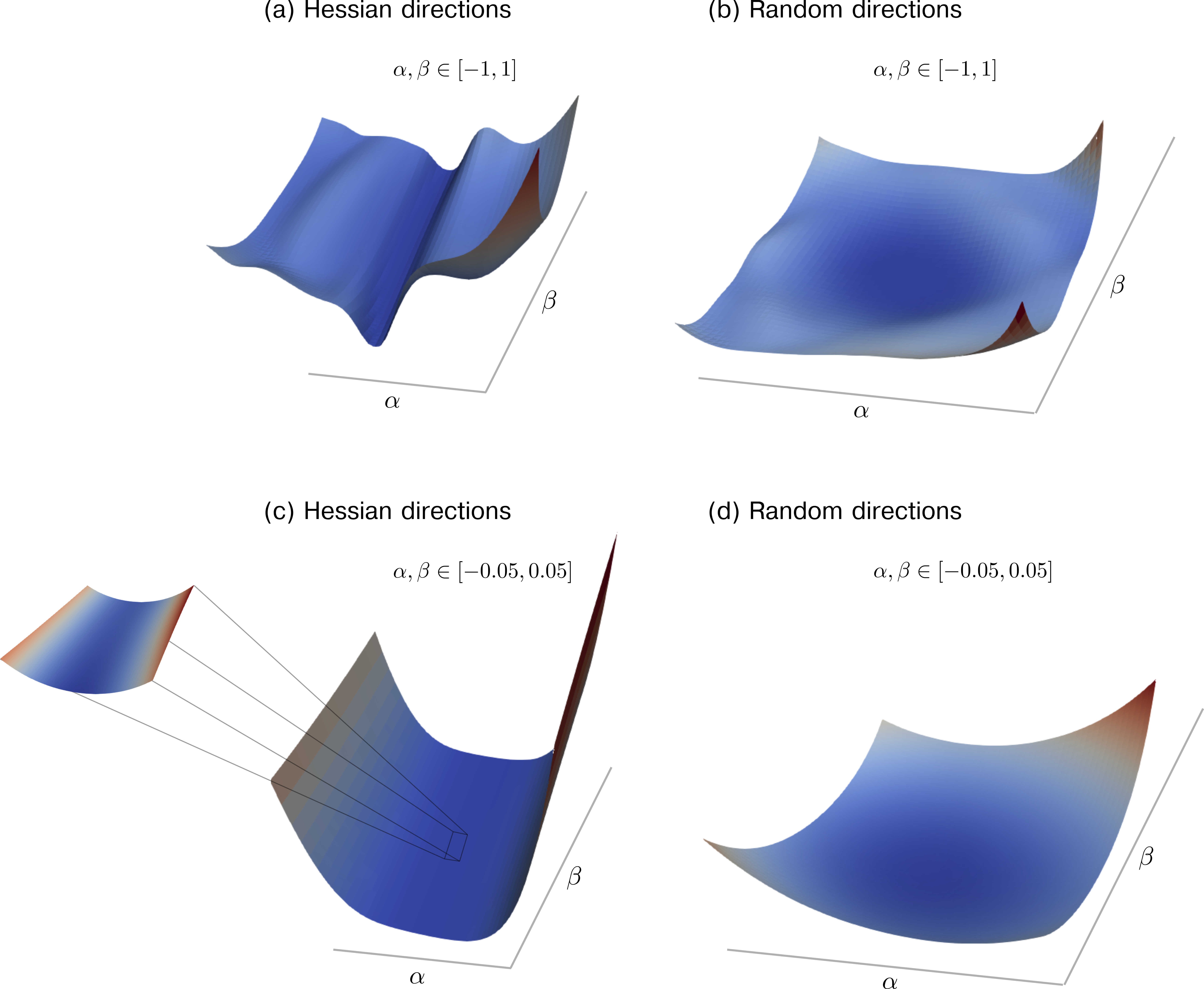
The image contains four 3D surface plots comparing function behavior under Hessian directions and random directions. Each plot uses α and β parameters with distinct value ranges, visualized through color gradients and surface topography.
### Components/Axes
1. **Axes Labels**:
- All plots use α (x-axis) and β (y-axis) parameters.
- Z-axis represents function value (no explicit label).
2. **Parameter Ranges**:
- **(a) & (b)**: α, β ∈ [-1, 1]
- **(c) & (d)**: α, β ∈ [-0.05, 0.05]
3. **Color Gradient**:
- Blue-to-red gradient (no explicit legend; inferred to represent function magnitude).
4. **Surface Features**:
- **(a)**: Saddle-shaped surface with sharp curvature.
- **(b)**: Smooth surface with gentle curvature.
- **(c)**: Narrow saddle shape with visible directional vectors.
- **(d)**: Smooth surface with subtle curvature.
### Detailed Analysis
1. **Plot (a) - Hessian Directions (α, β ∈ [-1,1])**:
- Saddle shape indicates mixed curvature (positive and negative eigenvalues).
- Color gradient shows rapid value changes near the saddle point.
- No directional vectors or annotations.
2. **Plot (b) - Random Directions (α, β ∈ [-1,1])**:
- Uniformly smooth surface with minimal curvature.
- Color gradient is more gradual compared to (a).
- No directional vectors or annotations.
3. **Plot (c) - Hessian Directions (α, β ∈ [-0.05,0.05])**:
- Narrow saddle shape with directional vectors (arrows) pointing toward critical points.
- Color gradient highlights localized curvature changes.
- Vectors suggest gradient flow toward the saddle's center.
4. **Plot (d) - Random Directions (α, β ∈ [-0.05,0.05])**:
- Uniformly smooth surface with minimal curvature.
- Color gradient is consistent across the range.
- No directional vectors or annotations.
### Key Observations
1. **Curvature Differences**:
- Hessian directions (a,c) produce saddle shapes, while random directions (b,d) yield smooth surfaces.
2. **Scale Sensitivity**:
- Narrower ranges (c,d) emphasize local curvature, while wider ranges (a,b) show global behavior.
3. **Directional Vectors**:
- Only present in (c), indicating gradient flow toward critical points.
4. **Color Correlation**:
- Red regions likely represent higher function values; blue regions lower values (inferred from gradient).
### Interpretation
1. **Hessian vs. Random Directions**:
- Hessian directions (a,c) reveal critical curvature properties (saddle points), while random directions (b,d) show averaged, smooth behavior.
2. **Parameter Range Impact**:
- Wider ranges (a,b) capture global function structure, while narrower ranges (c,d) focus on local curvature near critical points.
3. **Directional Vectors in (c)**:
- Arrows suggest gradient descent paths converging at the saddle point, highlighting optimization challenges in such regions.
4. **Function Behavior**:
- The saddle shapes imply the presence of inflection points or saddle points in the function's landscape, critical for optimization algorithms.
### Spatial Grounding
- All plots share consistent axis labeling (α, β) and color gradient direction.
- Plot (c) uniquely includes directional vectors anchored to the surface, spatially grounding gradient flow.
### Content Details
- No explicit numerical values or legends are provided; analysis relies on visual interpretation of curvature, color gradients, and vector directions.
- All plots use the same α-β parameter space but differ in surface topology and directional annotations.