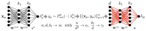
## Neural Network Diagram: Forward and Backward Propagation ### Overview The image depicts a neural network diagram illustrating forward and backward propagation. The diagram is split into two sections, showing the network's state before and after training. The left side represents the initial state with gray connections, while the right side represents the trained state with red connections. ### Components/Axes * **Nodes:** The diagram features nodes arranged in layers. The number of nodes in each layer varies. * **Connections:** Lines connecting the nodes represent the weights between neurons. The color of the lines changes from gray (initial state) to red (trained state). * **Labels:** * Input Layer: x_μ * Hidden Layers: d, k₁, k₂ * Output Layer: λ_μ⁰ (left), λ_μ (right) * Weights: w⁽¹⁾⁰, w⁽²⁾⁰ (left), w⁽¹⁾, w⁽²⁾ (right), v⁰ (left), v (right) * **Equations:** * Left side: λ_μ⁰ → y_μ ~ P_out(· | λ_μ⁰) * Center: {(x_μ, y_μ)}_μ=1ⁿ * Right side: n, d, k_l → ∞ with n/d² → α, k_l/d → γ_l ### Detailed Analysis **Left Side (Initial State):** * The input layer is labeled x_μ and has approximately 5 nodes. * The first hidden layer is labeled 'd' and also has approximately 5 nodes. * The second hidden layer is labeled 'k₁' and has approximately 4 nodes. * The third hidden layer is labeled 'k₂' and has approximately 5 nodes. * The output layer is labeled λ_μ⁰ and has a single node. * The connections between the layers are gray, indicating the initial, untrained state of the network. * The weights associated with the connections are labeled w⁽¹⁾⁰, w⁽²⁾⁰, and v⁰. **Right Side (Trained State):** * The input layer is labeled 'd' and has approximately 5 nodes. * The first hidden layer is labeled 'k₁' and has approximately 4 nodes. * The second hidden layer is labeled 'k₂' and has approximately 5 nodes. * The output layer is labeled λ_μ and has a single node. * The connections between the layers are red, indicating the trained state of the network. * The weights associated with the connections are labeled w⁽¹⁾, w⁽²⁾, and v. **Equations and Relationships:** * The equation λ_μ⁰ → y_μ ~ P_out(· | λ_μ⁰) describes the forward pass, where λ_μ⁰ is the initial output, y_μ is the target output, and P_out is the output distribution. * The term {(x_μ, y_μ)}_μ=1ⁿ represents the training dataset consisting of input-output pairs. * The equation n, d, k_l → ∞ with n/d² → α, k_l/d → γ_l describes the asymptotic behavior of the network as the number of training samples (n), input dimension (d), and hidden layer sizes (k_l) approach infinity. α and γ_l are constants. ### Key Observations * The color change from gray to red signifies the transition from an untrained to a trained network. * The diagram illustrates the flow of information from the input layer to the output layer during both forward and backward propagation. * The equations provide a mathematical description of the network's behavior and training process. ### Interpretation The diagram illustrates the fundamental concept of training a neural network. The left side represents the initial, random state of the network, where the connections (weights) are untrained. The right side represents the trained network, where the connections have been adjusted to map the input data to the desired output. The equations describe the mathematical relationships between the input, output, and network parameters. The asymptotic behavior equation suggests that the network's performance improves as the size of the network and the amount of training data increase. The diagram effectively visualizes the transformation of a neural network from a random mapping to a learned mapping through the process of training.

## Diagram: Neural Network Architectures & Asymptotic Behavior ### Overview The image presents two diagrams illustrating neural network architectures alongside a mathematical expression describing their asymptotic behavior as the network size increases. The left diagram depicts a feedforward neural network, while the right diagram shows a different network structure. The central text block provides a mathematical relationship between network parameters and their limits. ### Components/Axes The diagrams do not have traditional axes. Instead, they represent network layers with nodes (black circles) and connections (lines). The diagrams are labeled with variables representing input, weights, and output. * **Left Diagram Labels:** * `xµ`: Input layer. * `d`: Number of input features. * `k1`, `k2`: Number of nodes in hidden layers. * `w(0)`: Weights connecting the input layer to the first hidden layer. * `w(20)`: Weights connecting the first hidden layer to the second hidden layer. * `v(0)`: Weights connecting the second hidden layer to the output layer. * `λµ0`: Output of the first hidden layer. * `λµ`: Output of the second hidden layer. * **Right Diagram Labels:** * `d`: Number of input features. * `k1`, `k2`: Number of nodes in hidden layers. * `w(0)`: Weights connecting the input layer to the first hidden layer. * `w(2)`: Weights connecting the first hidden layer to the output layer. * `λµ`: Output layer. * `v`: Output. * **Central Text Block:** * `yµ0 ≈ Pout(·|λµ)` * `{(xµ, yµ)n}fµ=1→1` * `n, d, k1 → ∞ with n/d² → α, k1/d → η` ### Detailed Analysis or Content Details **Left Diagram:** The left diagram shows a feedforward neural network with an input layer (`xµ`) connected to two hidden layers (`λµ0`, `λµ`) and finally to an output layer (`λµ`). The connections between layers are represented by lines, indicating weighted connections (`w(0)`, `w(20)`, `v(0)`). The number of nodes in each layer is denoted by `d`, `k1`, and `k2`. **Right Diagram:** The right diagram depicts a different network structure. The input layer (`d`) is fully connected to a hidden layer (`k1`), and this hidden layer is fully connected to the output layer (`λµ`). The weights connecting these layers are denoted by `w(0)` and `w(2)`. The output is represented by `v`. **Central Text Block:** The text block presents a mathematical relationship. * `yµ0 ≈ Pout(·|λµ)`: This equation suggests that the output of the first hidden layer (`yµ0`) is approximately equal to the probability distribution `Pout` conditioned on `λµ`. * `{(xµ, yµ)n}fµ=1→1`: This notation indicates a sequence of data points `(xµ, yµ)` with `n` samples, where `fµ=1` suggests a limit or convergence. * `n, d, k1 → ∞ with n/d² → α, k1/d → η`: This statement describes the asymptotic behavior of the network as the number of samples (`n`), input features (`d`), and nodes in the first hidden layer (`k1`) approach infinity. The ratios `n/d²` and `k1/d` converge to constants `α` and `η`, respectively. ### Key Observations * The diagrams illustrate different neural network architectures. The left diagram shows a deeper network with multiple hidden layers, while the right diagram shows a shallower network. * The mathematical expression describes the behavior of these networks as their size increases. The convergence of `n/d²` to `α` and `k1/d` to `η` suggests that the network's performance depends on the relationship between the number of samples, input features, and hidden layer nodes. * The notation used in the mathematical expression is standard in the field of neural networks and statistical learning. ### Interpretation The image demonstrates the relationship between neural network architecture, network size, and asymptotic behavior. The diagrams visually represent the flow of information through the network, while the mathematical expression provides a formal description of how the network's performance changes as its size increases. The convergence of the ratios `n/d²` and `k1/d` suggests that there is an optimal balance between the number of samples, input features, and hidden layer nodes for achieving good performance. The notation `Pout(·|λµ)` suggests a probabilistic interpretation of the network's output, where the network is learning to estimate a probability distribution. The diagrams and the mathematical expression together provide a comprehensive understanding of the fundamental principles underlying neural network design and training.

## Diagram: Neural Network Architecture Transformation with Asymptotic Analysis ### Overview The image displays a technical diagram illustrating the transformation of a neural network's architecture and output distribution under asymptotic conditions (as dimensions grow infinitely large). It consists of two neural network schematics (left and right) connected by a central mathematical expression describing a limiting process. The diagram is likely from a theoretical machine learning or statistical physics paper discussing the behavior of wide neural networks. ### Components/Axes The diagram is composed of three main regions arranged horizontally: 1. **Left Region (Initial Network):** * A fully-connected neural network diagram with an input layer, two hidden layers, and an output node. * **Labels (Top):** `d`, `k₁`, `k₂` (indicating the widths of the input layer, first hidden layer, and second hidden layer, respectively). * **Labels (Nodes):** Input vector `x_u`. Output node labeled `λ_u⁰`. * **Labels (Connections):** Weight matrices `W^(1)` and `W^(2)`. A bias or scaling term `γ⁰` is noted near the output. * **Visual Style:** All connections are drawn in **black**. 2. **Central Region (Mathematical Transformation):** * A sequence of mathematical expressions connected by arrows (`⇒`), defining a limiting process and a distributional relationship. * **Transcription:** `λ_u⁰ ⇒ y_u ~ P_out⁰(· | λ_u⁰) ⇒ {(x_u, y_u)}_{u=1}^n` `n, d, k₁ → ∞ with d/n → α, k₁/d → γ₁` 3. **Right Region (Final/Transformed Network):** * A neural network diagram structurally identical to the left one. * **Labels (Top):** `d`, `k₁`, `k₂` (same as left). * **Labels (Nodes):** Input vector `x_u`. Output node labeled `λ_u`. * **Labels (Connections):** Weight matrices `W^(1)` and `W^(2)`. A vector `v` is noted near the output. * **Visual Style:** All connections are drawn in **red**. ### Detailed Analysis * **Network Structure:** Both networks have an input dimension `d`, a first hidden layer of width `k₁`, a second hidden layer of width `k₂`, and a scalar output. The architecture is `d -> k₁ -> k₂ -> 1`. * **Transformation Process (Central Text):** 1. The initial network output `λ_u⁰` is used to generate a target value `y_u` by sampling from a conditional output distribution `P_out⁰(· | λ_u⁰)`. 2. This process creates a dataset of `n` samples: `{(x_u, y_u)}_{u=1}^n`. 3. The key asymptotic limit is then defined: the sample size `n`, input dimension `d`, and first hidden layer width `k₁` all tend to infinity (`→ ∞`). Their relative scaling is controlled by two constants: * `α = d/n` (the ratio of input dimension to sample size). * `γ₁ = k₁/d` (the ratio of first hidden layer width to input dimension). * **Visual Change:** The primary visual difference between the left and right networks is the color of the connection lines (black vs. red). This likely symbolizes a change in the state of the network's parameters (weights) – for instance, from initialization (black) to trained/optimized values (red) – after undergoing the process described in the central limit. ### Key Observations 1. **Color-Coded State Change:** The shift from black to red connections is the most salient visual cue, explicitly differentiating two states of the same network architecture. 2. **Asymptotic Framework:** The diagram is fundamentally about the **theoretical behavior** of the network in a specific high-dimensional limit (`n, d, k₁ → ∞`), not a specific finite instance. 3. **Parameterization:** The scaling constants `α` and `γ₁` are critical. They define the "shape" of the high-dimensional limit, which is a common technique in the theoretical analysis of neural networks (e.g., in the Neural Tangent Kernel or mean-field theory literature). 4. **Output Evolution:** The output node's label changes from `λ_u⁰` (left) to `λ_u` (right), indicating the network's final output after the transformation. The intermediate variable `y_u` represents the training target derived from the initial network. ### Interpretation This diagram illustrates a theoretical framework for studying how a randomly initialized neural network (left, with parameters in state `⁰`) can be transformed into a trained network (right) through a process that involves generating labels from its own initial outputs and then considering an infinite-size limit. * **What it represents:** It models a scenario where a network's initial predictions are used to create a synthetic dataset, and then the network is trained on this data. The diagram focuses on the mathematical limit where the network and dataset sizes become very large in a proportional way (`α`, `γ₁` fixed). * **Relationship between elements:** The central equations are the bridge. They show that the final network (red) is the result of applying an empirical risk minimization (training) process on the dataset `{(x_u, y_u)}` generated from the initial network (black). The asymptotic conditions allow for a precise, often simplified, mathematical analysis of the trained network's properties (like its output `λ_u` or its generalization error). * **Underlying Concept:** This is characteristic of research in the **theory of deep learning**, aiming to understand why overparameterized networks generalize well. The specific limit (`d/n → α`, `k₁/d → γ₁`) suggests an analysis where both the number of parameters and the number of samples are large, but their ratios are controlled. The red network likely represents the "limit" of the trained network as these dimensions go to infinity, a state that can often be described by deterministic equations (like kernel methods or differential equations) despite the randomness in finite instances.

## Neural Network Architecture Diagram: Two-Layer Feedforward Networks with Parameter Scaling ### Overview The image depicts two interconnected neural network architectures with mathematical annotations. The left side shows a standard feedforward network with input `x_μ`, hidden layers, and output `y_μ`, while the right side shows a modified network with output `λ_μ`. Equations describe parameter relationships and asymptotic behavior. ### Components/Axes 1. **Left Network (Black Lines)** - Input: `x_μ` (dimension `d`) - Hidden Layers: - First layer weights: `W^(1)_0` (dimension `d × k₁`) - Second layer weights: `W^(2)_0` (dimension `k₁ × k₂`) - Output: `y_μ` (dimension `k₂`) - Probability: `P^0_out(·|λ^0_μ)` (conditional distribution) - Equation: `y_μ ~ P^0_out(·|λ^0_μ)` 2. **Right Network (Red Lines)** - Input: `x_μ` (same as left network) - Hidden Layers: - First layer weights: `W^(1)` (dimension `d × k₁`) - Second layer weights: `W^(2)` (dimension `k₁ × k₂`) - Output: `λ_μ` (dimension `k₂`) - Equation: `λ_μ` derived from `y_μ` through transformation 3. **Parameter Relationships** - Asymptotic scaling: `n, d, k_l → ∞` with: - `n/d² → α` (signal-to-noise ratio) - `k_l/d → γ_l` (width-to-depth ratio) ### Detailed Analysis - **Left Network Flow**: `x_μ` → `W^(1)_0` → `W^(2)_0` → `λ^0_μ` → `y_μ` - Input dimension: `d` - Hidden layer dimensions: `k₁` (first layer), `k₂` (second layer) - Output dimension: `k₂` - **Right Network Flow**: `x_μ` → `W^(1)` → `W^(2)` → `λ_μ` - Maintains same dimensionality as left network - Output `λ_μ` represents transformed version of `y_μ` - **Key Equations**: 1. `y_μ ~ P^0_out(·|λ^0_μ)`: Output distribution conditioned on latent variable 2. Asymptotic scaling laws: - `n/d² → α`: Sample complexity scaling - `k_l/d → γ_l`: Network width scaling ### Key Observations 1. **Architectural Symmetry**: Both networks share identical dimensionality structure (`d → k₁ → k₂`) 2. **Weight Differentiation**: - Left network uses subscripted weights (`W^(1)_0`, `W^(2)_0`) - Right network uses standard weights (`W^(1)`, `W^(2)`) 3. **Latent Variable Transformation**: - `λ^0_μ` serves as intermediate representation - `λ_μ` appears to be a modified version of `λ^0_μ` 4. **Scaling Regimes**: - `α` controls signal strength relative to noise - `γ_l` governs network expressivity ### Interpretation This diagram illustrates a theoretical analysis of neural network behavior under specific scaling regimes. The left network represents a baseline architecture with fixed initialization (`_0` subscripts), while the right network shows a modified version with potentially learned weights. The equations suggest: 1. **Capacity Analysis**: The `n/d² → α` relationship indicates how sample size scales with input dimension to maintain signal quality. 2. **Expressivity Tradeoff**: The `k_l/d → γ_l` ratio shows how network width grows relative to input size. 3. **Latent Space Dynamics**: The transformation from `λ^0_μ` to `λ_μ` implies a non-linear processing step that could represent: - Regularization - Feature extraction - Loss function optimization The red/black color coding emphasizes the architectural relationship between the two networks, suggesting the right network is a variant or optimized version of the left. The asymptotic analysis implies this is a theoretical study of network behavior in high-dimensional limits, relevant for understanding generalization bounds and capacity tradeoffs in deep learning.