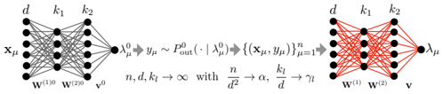
## Neural Network Architecture Diagram: Two-Layer Feedforward Networks with Parameter Scaling ### Overview The image depicts two interconnected neural network architectures with mathematical annotations. The left side shows a standard feedforward network with input `x_μ`, hidden layers, and output `y_μ`, while the right side shows a modified network with output `λ_μ`. Equations describe parameter relationships and asymptotic behavior. ### Components/Axes 1. **Left Network (Black Lines)** - Input: `x_μ` (dimension `d`) - Hidden Layers: - First layer weights: `W^(1)_0` (dimension `d × k₁`) - Second layer weights: `W^(2)_0` (dimension `k₁ × k₂`) - Output: `y_μ` (dimension `k₂`) - Probability: `P^0_out(·|λ^0_μ)` (conditional distribution) - Equation: `y_μ ~ P^0_out(·|λ^0_μ)` 2. **Right Network (Red Lines)** - Input: `x_μ` (same as left network) - Hidden Layers: - First layer weights: `W^(1)` (dimension `d × k₁`) - Second layer weights: `W^(2)` (dimension `k₁ × k₂`) - Output: `λ_μ` (dimension `k₂`) - Equation: `λ_μ` derived from `y_μ` through transformation 3. **Parameter Relationships** - Asymptotic scaling: `n, d, k_l → ∞` with: - `n/d² → α` (signal-to-noise ratio) - `k_l/d → γ_l` (width-to-depth ratio) ### Detailed Analysis - **Left Network Flow**: `x_μ` → `W^(1)_0` → `W^(2)_0` → `λ^0_μ` → `y_μ` - Input dimension: `d` - Hidden layer dimensions: `k₁` (first layer), `k₂` (second layer) - Output dimension: `k₂` - **Right Network Flow**: `x_μ` → `W^(1)` → `W^(2)` → `λ_μ` - Maintains same dimensionality as left network - Output `λ_μ` represents transformed version of `y_μ` - **Key Equations**: 1. `y_μ ~ P^0_out(·|λ^0_μ)`: Output distribution conditioned on latent variable 2. Asymptotic scaling laws: - `n/d² → α`: Sample complexity scaling - `k_l/d → γ_l`: Network width scaling ### Key Observations 1. **Architectural Symmetry**: Both networks share identical dimensionality structure (`d → k₁ → k₂`) 2. **Weight Differentiation**: - Left network uses subscripted weights (`W^(1)_0`, `W^(2)_0`) - Right network uses standard weights (`W^(1)`, `W^(2)`) 3. **Latent Variable Transformation**: - `λ^0_μ` serves as intermediate representation - `λ_μ` appears to be a modified version of `λ^0_μ` 4. **Scaling Regimes**: - `α` controls signal strength relative to noise - `γ_l` governs network expressivity ### Interpretation This diagram illustrates a theoretical analysis of neural network behavior under specific scaling regimes. The left network represents a baseline architecture with fixed initialization (`_0` subscripts), while the right network shows a modified version with potentially learned weights. The equations suggest: 1. **Capacity Analysis**: The `n/d² → α` relationship indicates how sample size scales with input dimension to maintain signal quality. 2. **Expressivity Tradeoff**: The `k_l/d → γ_l` ratio shows how network width grows relative to input size. 3. **Latent Space Dynamics**: The transformation from `λ^0_μ` to `λ_μ` implies a non-linear processing step that could represent: - Regularization - Feature extraction - Loss function optimization The red/black color coding emphasizes the architectural relationship between the two networks, suggesting the right network is a variant or optimized version of the left. The asymptotic analysis implies this is a theoretical study of network behavior in high-dimensional limits, relevant for understanding generalization bounds and capacity tradeoffs in deep learning.