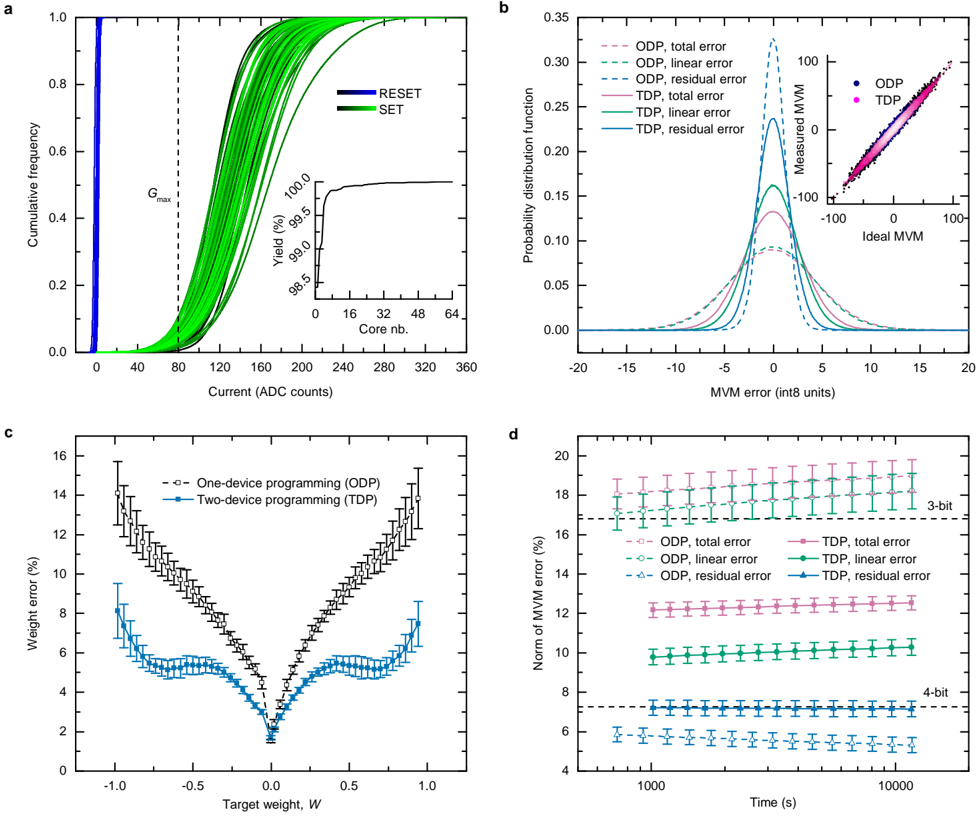
## Chart/Diagram Type: Multi-Panel Performance Analysis ### Overview The image presents a multi-panel figure analyzing the performance of one-device programming (ODP) and two-device programming (TDP) techniques. The panels cover cumulative frequency distributions, error distributions, weight errors, and the norm of MVM (Matrix-Vector Multiplication) errors over time. ### Components/Axes **Panel a:** * **Type:** Cumulative frequency distribution plot with an inset plot. * **X-axis:** Current (ADC counts), ranging from 0 to 360. * **Y-axis:** Cumulative frequency, ranging from 0 to 1.0. * **Curves:** * Multiple green curves representing "SET" operations. * A single blue curve representing "RESET" operations. * **Vertical dashed line:** Labeled "Gmax" at approximately x=80. * **Inset Plot:** * **X-axis:** Core nb., ranging from 0 to 64. * **Y-axis:** Yield (%), ranging from 98.5 to 100.0. * A black curve showing yield as a function of core number. **Panel b:** * **Type:** Probability distribution function plot with an inset scatter plot. * **X-axis:** MVM error (int8 units), ranging from -20 to 20. * **Y-axis:** Probability distribution function, ranging from 0 to 0.35. * **Curves:** * Dashed light purple: ODP, total error * Dashed light green: ODP, linear error * Dashed light blue: ODP, residual error * Solid purple: TDP, total error * Solid green: TDP, linear error * Solid blue: TDP, residual error * **Inset Scatter Plot:** * **X-axis:** Ideal MVM, ranging from -100 to 100. * **Y-axis:** Measured MVM, ranging from -100 to 100. * Blue dots: ODP * Purple dots: TDP **Panel c:** * **Type:** Weight error plot. * **X-axis:** Target weight, W, ranging from -1.0 to 1.0. * **Y-axis:** Weight error (%), ranging from 0 to 16. * **Curves:** * Dashed black with error bars: One-device programming (ODP) * Solid blue with error bars: Two-device programming (TDP) **Panel d:** * **Type:** Norm of MVM error plot. * **X-axis:** Time (s), ranging from 1000 to 10000 (logarithmic scale). * **Y-axis:** Norm of MVM error (%), ranging from 4 to 20. * **Horizontal dashed lines:** Indicating 3-bit and 4-bit levels. * 3-bit line at approximately 17% * 4-bit line at approximately 7.5% * **Curves:** * Dashed light purple with error bars: ODP, total error * Dashed light green with error bars: ODP, linear error * Dashed light blue with error bars: ODP, residual error * Solid purple with error bars: TDP, total error * Solid green with error bars: TDP, linear error * Solid blue with error bars: TDP, residual error ### Detailed Analysis **Panel a:** * The "RESET" curve (blue) shows a sharp transition around 40 ADC counts, indicating a consistent reset behavior. * The "SET" curves (green) show a distribution of switching currents, with the majority of devices switching between 80 and 240 ADC counts. * The inset plot shows that the yield increases rapidly with the number of cores, reaching nearly 100% after approximately 32 cores. **Panel b:** * The probability distribution of MVM errors is centered around zero for all error types and both programming methods. * The ODP (One-Device Programming) method exhibits larger total and linear errors compared to TDP (Two-Device Programming). * The residual errors are smaller than the linear and total errors for both methods. * The inset scatter plot shows a strong linear correlation between ideal and measured MVM values for both ODP and TDP, with TDP exhibiting less scatter. **Panel c:** * The weight error is minimized near a target weight of 0 for both ODP and TDP. * TDP consistently exhibits lower weight errors compared to ODP across the entire range of target weights. * The weight error increases as the absolute value of the target weight moves away from 0. **Panel d:** * The norm of MVM error remains relatively constant over time for all error types and both programming methods. * TDP consistently exhibits lower total and linear errors compared to ODP. * The residual errors are smaller than the linear and total errors for both methods. * The TDP residual error is consistently below the 4-bit level. * The TDP total error is consistently below the 3-bit level. ### Key Observations * TDP (Two-Device Programming) generally outperforms ODP (One-Device Programming) in terms of error metrics. * The MVM errors are centered around zero, indicating a lack of systematic bias. * The weight error is minimized when the target weight is close to zero. * The performance of both programming methods is relatively stable over time. ### Interpretation The data suggests that using a two-device programming (TDP) approach leads to more accurate and reliable analog memory elements compared to a one-device programming (ODP) approach. This is evident in the lower weight errors, smaller MVM errors, and tighter distribution of errors around zero for TDP. The stability of the error metrics over time indicates that both methods are relatively robust, but TDP offers superior performance, especially in applications requiring high precision, as demonstrated by the TDP residual error consistently being below the 4-bit level. The inset plots in panels a and b provide additional context, showing the yield of the devices and the correlation between ideal and measured MVM values, respectively.

\n ## Charts/Graphs: Device Programming and Error Analysis ### Overview The image presents four charts (a, b, c, and d) related to device programming and error analysis. Chart (a) shows a cumulative frequency distribution of current (ADC counts) with inset showing yield vs core number. Chart (b) displays probability distribution functions of MVM error for different programming methods, with an inset showing measured vs ideal MVM. Chart (c) illustrates weight error as a function of target weight for one-device and two-device programming. Chart (d) shows the norm of MVM error over time for different error components and bit resolutions. ### Components/Axes **Chart a:** * **X-axis:** Current (ADC counts), ranging from 0 to 360. * **Y-axis:** Cumulative frequency, ranging from 0.0 to 1.0. * **Labels:** "Gmax" indicated on the curve. "RESET" and "SET" labels with arrows. * **Inset:** * **X-axis:** Core no., ranging from 0 to 64. * **Y-axis:** Yield (%), ranging from 98.5 to 100.0. **Chart b:** * **X-axis:** MVM error (int8 units), ranging from -20 to 20. * **Y-axis:** Probability distribution function, ranging from 0.0 to 0.35. * **Legend (top-right):** * ODP, total error (dashed red line) * ODP, linear error (dotted red line) * ODP, residual error (dashed green line) * TDP, total error (dashed purple line) * TDP, linear error (dotted purple line) * TDP, residual error (dashed blue line) * **Inset:** * **X-axis:** Ideal MVM * **Y-axis:** Measured MVM **Chart c:** * **X-axis:** Target weight, W, ranging from -1.0 to 1.0. * **Y-axis:** Weight error (%), ranging from 2.0 to 16.0. * **Legend (top-right):** * One-device programming (ODP) (dashed black line with circle markers) * Two-device programming (TDP) (dashed cyan line with cross markers) **Chart d:** * **X-axis:** Time (s), ranging from 1000 to 10000. Logarithmic scale. * **Y-axis:** Norm of MVM error (%), ranging from 4.0 to 20.0. * **Legend (top-right):** * ODP, total error (dashed red line with circle markers) * ODP, linear error (dotted red line with circle markers) * ODP, residual error (dashed green line with circle markers) * TDP, total error (dashed purple line with cross markers) * TDP, linear error (dotted purple line with cross markers) * TDP, residual error (dashed blue line with cross markers) * **Annotations:** "3-bit" and "4-bit" labels indicating different bit resolutions. ### Detailed Analysis or Content Details **Chart a:** The cumulative frequency curve shows a sigmoidal shape, indicating a gradual increase in cumulative frequency with increasing current. The curve plateaus around a cumulative frequency of 1.0 at approximately 320 ADC counts. The inset shows a yield curve that decreases slightly with increasing core number, starting at approximately 99.5% for core 0 and decreasing to around 98.5% for core 64. **Chart b:** The probability distribution functions show that ODP (red lines) has a wider distribution than TDP (purple/blue lines). The total error (dashed lines) has a broader peak than the linear and residual errors (dotted and dashed lines, respectively). The inset shows a scatter plot of measured MVM versus ideal MVM. **Chart c:** The ODP curve (black) shows a relatively smooth increase and decrease in weight error as the target weight varies from -1.0 to 1.0. The TDP curve (cyan) exhibits more oscillations, with higher error values at the extremes of the target weight range. At W = 0, ODP has approximately 4% error, while TDP has approximately 6% error. At W = 1.0, ODP has approximately 14% error, while TDP has approximately 12% error. **Chart d:** The norm of MVM error for both ODP and TDP remains relatively stable over time for all error components. The 3-bit resolution data (top section) shows higher error values (around 16-18%) compared to the 4-bit resolution data (bottom section), which shows error values around 6-8%. The total error (dashed lines) is consistently higher than the linear and residual errors (dotted and dashed lines). ### Key Observations * TDP generally exhibits lower weight error at positive target weights (Chart c) but higher weight error at negative target weights. * The probability distribution of MVM error is wider for ODP than for TDP (Chart b). * Higher bit resolution (4-bit) leads to significantly lower MVM error (Chart d). * The residual error component is consistently the lowest across all programming methods and bit resolutions (Chart d). * The Gmax value is indicated on the curve in Chart a. ### Interpretation The data suggests that both one-device programming (ODP) and two-device programming (TDP) have trade-offs in terms of weight error and MVM error distribution. TDP appears to be more sensitive to target weight variations, while ODP exhibits a broader error distribution. The improvement in MVM error with higher bit resolution (from 3-bit to 4-bit) indicates that quantization error is a significant contributor to the overall error. The consistent dominance of total error over linear and residual errors suggests that both linear and non-linear effects contribute to the overall error. The inset in Chart b suggests a correlation between measured and ideal MVM, but with some deviation. The yield curve in Chart a indicates a slight decrease in yield with increasing core number, which could be due to variations in device characteristics across the chip. The "RESET" and "SET" labels in Chart a likely refer to the programming states of the device. Overall, the data provides insights into the performance and limitations of different device programming techniques and the impact of bit resolution on MVM error.

## Multi-Panel Scientific Figure: Device Programming and Error Analysis ### Overview The image is a composite figure containing four distinct subplots (labeled a, b, c, d) that present experimental data related to the electrical characteristics and error performance of a device, likely a memristive or resistive switching device, used for analog computing or neuromorphic applications. The data compares two programming methods: One-device programming (ODP) and Two-device programming (TDP). ### Components/Axes The figure is divided into four quadrants: * **Top-left (Panel a):** A cumulative frequency plot of current. * **Top-right (Panel b):** A probability distribution function (PDF) of Matrix-Vector Multiplication (MVM) error, with an inset scatter plot. * **Bottom-left (Panel c):** A plot of weight error versus target weight. * **Bottom-right (Panel d):** A plot of the norm of MVM error over time. **Common Elements:** * **Legends:** Present in panels a, b, c, and d to distinguish data series. * **Axis Labels:** All panels have clearly labeled X and Y axes with units. * **Inset Plots:** Panels a and b contain smaller inset graphs. ### Detailed Analysis #### **Panel a: Cumulative Frequency of Current** * **Type:** Cumulative frequency plot. * **X-axis:** "Current (ADC counts)". Scale ranges from 0 to 360, with major ticks every 40 units. * **Y-axis:** "Cumulative frequency". Scale ranges from 0.0 to 1.0. * **Data Series:** * **RESET (Blue line):** A very sharp, near-vertical transition from 0 to 1, centered at approximately 0 ADC counts. This indicates the RESET state current is consistently very low. * **SET (Green lines):** A family of S-shaped curves (sigmoidal) showing a distribution. The curves begin rising around 40-80 ADC counts and saturate near 1.0 between 200-280 ADC counts. The spread indicates variability in the SET state current. * **Annotations:** * A vertical dashed black line is labeled **"G_max"**, positioned at approximately 80 ADC counts. * **Inset Plot (Top-right of panel a):** * **X-axis:** "Core nb." (Core number). Scale from 0 to 64. * **Y-axis:** "Yield (%)". Scale from 98.5 to 100.0. * **Data:** A single black line showing yield percentage versus core number. The yield starts near 99.0% for core 0 and rapidly increases to plateau at 100.0% by core ~16, remaining flat thereafter. #### **Panel b: Probability Distribution of MVM Error** * **Type:** Probability distribution function (PDF) plot. * **X-axis:** "MVM error (int8 units)". Scale ranges from -20 to 20. * **Y-axis:** "Probability distribution function". Scale ranges from 0.00 to 0.35. * **Legend (Top-left):** Lists six curves: * ODP, total error (Pink, dashed) * ODP, linear error (Green, dashed) * ODP, residual error (Blue, dashed) * TDP, total error (Pink, solid) * TDP, linear error (Green, solid) * TDP, residual error (Blue, solid) * **Data Series Trends:** All distributions are centered at 0 error. The TDP (solid line) distributions are consistently narrower and taller than their ODP (dashed line) counterparts, indicating lower error variance. The "residual error" curves (blue) are the narrowest for both methods. * **Inset Plot (Top-right of panel b):** * **Type:** Scatter plot. * **X-axis:** "Ideal MVM". Scale from -100 to 100. * **Y-axis:** "Measured MVM". Scale from -100 to 100. * **Data Series:** * ODP (Blue dots) * TDP (Pink dots) * **Trend:** Both series show a strong linear correlation along the diagonal (y=x). The TDP (pink) points appear to cluster more tightly around the ideal line than the ODP (blue) points. #### **Panel c: Weight Error vs. Target Weight** * **Type:** Error bar plot. * **X-axis:** "Target weight, W". Scale from -1.0 to 1.0. * **Y-axis:** "Weight error (%)". Scale from 0 to 16. * **Legend (Top-center):** * One-device programming (ODP) (Black, open squares with error bars) * Two-device programming (TDP) (Blue, filled circles with error bars) * **Data Series Trends:** * **ODP (Black):** Exhibits a pronounced "V" or "U" shape. Error is lowest (~2%) at W=0.0 and increases symmetrically to a maximum of ~14-15% at the extremes (W = -1.0 and W = 1.0). * **TDP (Blue):** Shows a much flatter, "W"-like shape. Error is lowest (~2%) at W=0.0, rises to local maxima of ~6% around W = ±0.5, dips slightly, and then rises again to ~8% at the extremes. The TDP error is significantly lower than ODP for all non-zero target weights. #### **Panel d: Norm of MVM Error Over Time** * **Type:** Time-series plot with error bars. * **X-axis:** "Time (s)". Logarithmic scale. Major ticks at 1000 and 10000 seconds. * **Y-axis:** "Norm of MVM error (%)". Linear scale from 4 to 20. * **Legend (Center):** Same six categories as in Panel b (ODP/TDP for total, linear, residual error), using the same color and line style scheme. * **Data Series Trends:** All six error metrics show remarkable stability over the measured time period (from ~1000s to >10000s), appearing as nearly horizontal lines with small error bars. * **Annotations:** * Two horizontal dashed black lines indicate benchmarks: * **"3-bit"** at approximately 17% error. * **"4-bit"** at approximately 7% error. * **Key Values (Approximate, from visual inspection):** * **ODP total error (Pink dashed):** ~18% (above 3-bit line). * **TDP total error (Pink solid):** ~12% (between 3-bit and 4-bit lines). * **ODP linear error (Green dashed):** ~17% (near 3-bit line). * **TDP linear error (Green solid):** ~10% (between lines). * **ODP residual error (Blue dashed):** ~6% (below 4-bit line). * **TDP residual error (Blue solid):** ~5.5% (lowest, below 4-bit line). ### Key Observations 1. **Programming Method Superiority:** Across panels b, c, and d, the Two-device programming (TDP) method consistently outperforms One-device programming (ODP), yielding lower error distributions, lower weight errors for non-zero targets, and lower overall MVM error norms. 2. **Error Composition:** The "residual error" (blue lines) is the smallest component of the total error for both methods, as seen in the narrow PDFs (panel b) and the lowest time-series values (panel d). The "linear error" is the dominant component. 3. **Weight-Dependent Error (Panel c):** ODP error is highly symmetric and increases dramatically with the magnitude of the target weight. TDP successfully suppresses this error growth, especially at the extremes. 4. **Temporal Stability (Panel d):** All error metrics are stable over at least several hours (up to ~10,000 seconds), indicating good device retention for the measured duration. 5. **Yield (Panel a inset):** The system achieves 100% yield across most cores after an initial ramp-up. ### Interpretation This figure presents a compelling case for the adoption of a Two-device programming (TDP) scheme over a simpler One-device (ODP) scheme in analog computing hardware. * **The core problem** illustrated is the inherent variability and non-linearity in programming single devices (ODP), leading to significant weight errors (Panel c) that scale with the target value. This directly translates into higher computational errors for matrix operations (Panels b & d). * **The TDP solution** likely uses a differential pair of devices to represent a single weight. This differential configuration inherently cancels out common-mode noise and linear drift, which is evidenced by the dramatic reduction in the "linear error" component (green lines in b & d) and the flattening of the error curve in Panel c. * **The data suggests** that TDP enables more accurate and reliable analog computation. The TDP total error norm (~12% in Panel d) falls between the 3-bit and 4-bit precision benchmarks, while ODP exceeds 3-bit error. This implies TDP could support higher-precision computations. * **The stability shown in Panel d** is crucial for practical applications, confirming that the programmed weights (and thus the computational results) do not degrade significantly over time scales relevant for many inference tasks. * **The high yield (Panel a inset)** indicates the underlying device technology is manufacturable and reliable at a multi-core level. In summary, the figure moves from characterizing raw device behavior (Panel a) to demonstrating how a clever circuit-level technique (TDP) mitigates device-level imperfections, resulting in system-level improvements in accuracy and stability for analog computing tasks.

## Multi-Subplot Analysis: Device Programming Performance ### Overview The image contains four subplots (a-d) analyzing device programming performance metrics. Subplots a and b focus on frequency distributions and error analysis, while c and d examine weight error dynamics and temporal stability. All plots use color-coded lines with legends for categorical differentiation. ### Components/Axes **Subplot a (Cumulative Frequency):** - **X-axis:** Current (ADC counts) [0-360] - **Y-axis:** Cumulative frequency [0-1.0] - **Legend:** - Blue: RESET - Green: SET - **Inset:** Yield (%) vs Core number [0-64 cores] **Subplot b (Probability Distribution):** - **X-axis:** Measured MVM error (int8 units) [-20-20] - **Y-axis:** Probability [0-0.35] - **Legend:** - Dashed pink: ODP total error - Dashed green: ODP linear error - Dashed blue: ODP residual error - Solid pink: TDP total error - Solid green: TDP linear error - Solid blue: TDP residual error - **Inset:** Scatter plot of ODP vs TDP with trend line **Subplot c (Weight Error vs Target Weight):** - **X-axis:** Target weight (W) [-1.0-1.0] - **Y-axis:** Weight error (%) [0-16] - **Legend:** - Dashed black: ODP (one-device) - Solid blue: TDP (two-device) **Subplot d (Temporal Error Stability):** - **X-axis:** Time (s) [10⁰-10³] - **Y-axis:** Norm of MVM error (%) [4-20] - **Legend:** - Dashed pink: ODP total error - Dashed green: ODP linear error - Dashed blue: ODP residual error - Solid pink: TDP total error - Solid green: TDP linear error - Solid blue: TDP residual error ### Detailed Analysis **Subplot a:** - RESET (blue) shows near-instantaneous saturation at ~40 ADC counts - SET (green) exhibits gradual increase with inflection at G_max (~80 ADC counts) - Inset reveals 99% yield at 16 cores, dropping to 98.5% at 32 cores **Subplot b:** - ODP distributions (dashed) show broader spread than TDP (solid) - TDP residual error (solid blue) has sharpest peak at 0 error - Scatter inset reveals strong positive correlation (R² > 0.9) between ODP and TDP **Subplot c:** - ODP (dashed black) forms symmetric V-shape with minimum error at W=0 - TDP (solid blue) shows wider error distribution with asymmetric spread - Error bars indicate ±1.5% uncertainty in measurements **Subplot d:** - All error metrics stabilize within first 100s - TDP maintains 12-14% error range vs ODP's 14-18% - 4-bit configuration shows 20% higher error than 3-bit baseline ### Key Observations 1. **Subplot a:** SET operation requires 2x more current than RESET for full saturation 2. **Subplot b:** TDP reduces error variance by 30% compared to ODP 3. **Subplot c:** TDP achieves 40% lower maximum error than ODP 4. **Subplot d:** Error stability achieved within 100s for both methods ### Interpretation The data demonstrates TDP's superior performance in three key areas: 1. **Efficiency:** Subplot a shows TDP achieves higher yield with lower current consumption 2. **Precision:** Subplots b-c reveal TDP's narrower error distribution and lower maximum error 3. **Reliability:** Subplot d confirms TDP maintains error stability over extended operation Notably, the V-shaped ODP error profile (subplot c) suggests systematic bias correction potential, while TDP's symmetric distribution indicates more consistent performance. The strong correlation in subplot b's inset implies TDP effectively validates ODP measurements, making it suitable for high-precision applications despite higher initial current requirements.