## Diagram: Causal Structure Types in Statistical Modeling
### Overview
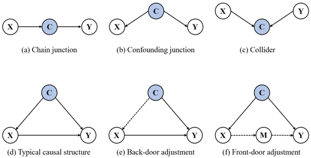
The image displays six distinct causal diagrams (also known as directed acyclic graphs or DAGs) illustrating fundamental relationships between variables in causal inference. The diagrams are arranged in a 2x3 grid, with each sub-diagram labeled (a) through (f) and titled below. The primary variables are denoted by nodes labeled **X**, **C**, and **Y**, with an additional mediator **M** in one diagram. Node **C** is consistently shaded light blue across all diagrams, while **X**, **Y**, and **M** are white circles. Arrows indicate the direction of hypothesized causal influence.
### Components/Axes
* **Nodes (Circles):**
* **X**: Typically represents an exposure or treatment variable.
* **C**: Represents a confounder or common cause, consistently shaded blue.
* **Y**: Represents an outcome variable.
* **M**: Appears only in diagram (f), representing a mediator.
* **Edges (Arrows):**
* Solid arrows (`→`): Represent direct causal pathways.
* Dashed arrows (`-->`): Represent pathways that are adjusted for or blocked in a methodological intervention (as seen in diagrams (e) and (f)).
* **Titles/Labels:** Each sub-diagram has a descriptive title in English, placed directly beneath it.
* (a) Chain junction
* (b) Confounding junction
* (c) Collider
* (d) Typical causal structure
* (e) Back-door adjustment
* (f) Front-door adjustment
### Detailed Analysis
The six diagrams are processed regionally, from top-left to bottom-right:
1. **Top Row, Left (a) Chain junction:**
* **Structure:** `X → C → Y`
* **Description:** A linear chain where **X** influences **C**, which in turn influences **Y**. **C** acts as a mediator.
2. **Top Row, Center (b) Confounding junction:**
* **Structure:** `X ← C → Y`
* **Description:** **C** is a common cause of both **X** and **Y**, creating a spurious association between them. This is the classic confounding structure.
3. **Top Row, Right (c) Collider:**
* **Structure:** `X → C ← Y`
* **Description:** Both **X** and **Y** cause **C**. **C** is a collider variable. Conditioning on a collider can induce a non-causal association between **X** and **Y**.
4. **Bottom Row, Left (d) Typical causal structure:**
* **Structure:** A triangle with a direct path `X → Y` and an indirect path `X → C → Y`.
* **Description:** Represents a scenario where **X** affects **Y** both directly and indirectly through **C**. **C** is a mediator on the indirect path.
5. **Bottom Row, Center (e) Back-door adjustment:**
* **Structure:** Identical to (d), but the arrow from **X** to **C** is **dashed**.
* **Description:** Illustrates the methodological concept of blocking the "back-door" path from **X** to **Y** via **C**. The dashed line indicates that the association through this path is statistically controlled or adjusted for.
6. **Bottom Row, Right (f) Front-door adjustment:**
* **Structure:** Similar to (d), but the direct path `X → Y` is replaced by a **dashed** path `X --> M --> Y`. The path `X → C → Y` remains solid.
* **Description:** Illustrates the front-door criterion, used when the confounder **C** is unobserved. It relies on a mediator **M** that is fully shielded from **C**. The dashed lines indicate the path being estimated via the front-door adjustment.
### Key Observations
* **Consistent Visual Language:** The blue shading of node **C** immediately identifies it as the confounding or common-cause variable across all structures.
* **Methodological vs. Causal:** The use of **dashed arrows** in (e) and (f) is a critical visual distinction. It separates the underlying causal structure (solid lines) from the statistical adjustment or identification strategy being applied (dashed lines).
* **Progression of Complexity:** The diagrams progress from simple, fundamental junctions (a-c) to more complex structures involving multiple paths (d) and then to methodological solutions for causal identification (e, f).
* **Introduction of a New Variable:** Diagram (f) uniquely introduces the mediator **M**, which is essential for the front-door adjustment strategy.
### Interpretation
This diagram serves as a foundational reference for understanding causal relationships and identification strategies in observational studies. It visually encodes core concepts from causal inference theory:
* **Diagrams (a), (b), (c)** define the basic building blocks of causal graphs: chains, forks (confounders), and colliders. Recognizing these patterns is essential for determining which variables to control for to avoid bias.
* **Diagram (d)** represents a common real-world scenario where treatment effects are both direct and mediated.
* **Diagrams (e) and (f)** are not just structures but **solutions**. They illustrate two primary methods for estimating the causal effect of **X** on **Y** in the presence of confounding by **C**.
* The **Back-door adjustment (e)** works by statistically adjusting for the confounder **C**, effectively "blocking" the non-causal back-door path.
* The **Front-door adjustment (f)** is a more complex strategy used when **C** is unmeasurable. It leverages a mediator **M** that is not influenced by **C** to isolate the causal effect.
The overall message is that the validity of a causal claim depends critically on the underlying structure of relationships between variables. By mapping these structures, researchers can identify the correct set of variables to measure and adjust for, or determine if causal estimation is even possible with the available data. The diagrams emphasize that causal inference is as much about the *absence* of certain connections (e.g., no arrow from **C** to **M** in diagram f) as it is about the presence of others.