## Line Graph: Gradient vs. x_t
### Overview
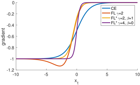
The image depicts a line graph comparing four distinct gradient behaviors across a range of x_t values (-10 to 10). The y-axis represents gradient values (-1.2 to 0), while the x-axis represents x_t. Four data series are plotted, each with unique curvature and inflection points, suggesting different functional relationships between x_t and gradient.
### Components/Axes
- **X-axis (x_t)**: Labeled "x_t", scaled from -10 to 10 in increments of 5.
- **Y-axis (gradient)**: Labeled "gradient", scaled from -1.2 to 0 in increments of 0.2.
- **Legend**: Positioned in the top-right corner, with four entries:
- **CE**: Blue line
- **FL γ=2**: Orange line
- **FL* γ=2, β=1**: Yellow line
- **FL* γ=4, β=0**: Purple line
- **Gridlines**: Faint horizontal and vertical lines at major axis intervals.
### Detailed Analysis
1. **CE (Blue Line)**:
- Starts at approximately -1.0 at x_t = -10.
- Gradually increases, reaching ~-0.2 by x_t = 0.
- Plateaus near 0 for x_t > 0.
2. **FL γ=2 (Orange Line)**:
- Begins at ~-1.0 at x_t = -10.
- Dips sharply to ~-1.1 at x_t ≈ -5.
- Rises steeply, crossing 0 at x_t ≈ 2.
- Plateaus near 0 for x_t > 2.
3. **FL* γ=2, β=1 (Yellow Line)**:
- Starts at ~-1.0 at x_t = -10.
- Rises gradually, crossing 0 at x_t ≈ 1.
- Plateaus near 0 for x_t > 1.
4. **FL* γ=4, β=0 (Purple Line)**:
- Starts at ~-1.0 at x_t = -10.
- Sharp ascent begins at x_t ≈ -3, crossing 0 at x_t ≈ 0.
- Remains flat at 0 for x_t > 0.
### Key Observations
- All lines converge at the lower bound (y ≈ -1.0) for x_t ≤ -10.
- The **FL* γ=4, β=0** (purple) line exhibits the steepest gradient increase, reaching 0 earliest (x_t ≈ 0).
- The **FL γ=2** (orange) line shows a unique dip below -1.0 before rising, unlike other series.
- **CE** (blue) and **FL* γ=2, β=1** (yellow) lines share similar shapes but differ in timing: CE reaches 0 at x_t ≈ 0, while the yellow line does so at x_t ≈ 1.
### Interpretation
The graph illustrates how gradient behavior varies with parameters γ (scaling factor) and β (offset). Higher γ values (e.g., γ=4) correlate with faster gradient increases, while β=0 eliminates delays in gradient ascent. The **FL γ=2** line’s anomalous dip suggests a transient negative gradient effect, potentially indicating a local minimum or damping effect. The **CE** line may represent a control or baseline scenario, showing gradual improvement without parameter-driven acceleration. These trends imply that parameter tuning (γ, β) critically influences gradient dynamics in the modeled system.