\n
## Diagram: Directed Graph and 3D Surface Plots
### Overview
The image contains two distinct parts labeled (a) and (b). Part (a) is a simple directed graph with two nodes and three labeled edges. Part (b) consists of two separate 3D surface plots, each visualizing a function over a triangular domain defined by binary vertex labels. The overall image appears to be from a technical or scientific document, likely illustrating concepts in systems theory, optimization, or mathematical modeling.
### Components/Axes
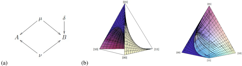
**Part (a) - Directed Graph:**
* **Nodes:** Two nodes labeled **A** (left) and **B** (right).
* **Edges (with labels and direction):**
* An edge from **A** to **B** labeled with the Greek letter **μ** (mu).
* An edge from **B** to **A** labeled with the Greek letter **ν** (nu).
* An edge pointing downward to node **B** labeled with the Greek letter **δ** (delta).
**Part (b) - 3D Surface Plots:**
* **Domain:** Both plots are defined over a triangular (simplex) domain.
* **Vertex Labels:** The vertices of the triangle are labeled with binary pairs:
* Bottom-left vertex: **[10]**
* Bottom-right vertex: **[11]**
* Top vertex: **[01]**
* A fourth label, **[00]**, is positioned at the bottom center of the left plot's triangle, suggesting it may represent the origin or a central point in the coordinate system.
* **Surfaces:** Each plot shows a 3D surface rendered with a colored mesh grid. The surfaces are bounded within the triangular domain.
* **Left Plot:** The surface appears to rise from the **[00]** and **[10]** regions towards a peak near the **[01]** vertex. The color gradient transitions from dark blue/purple in the lower regions to a lighter purple/pink at the higher points.
* **Right Plot:** The surface has a different curvature, appearing to form a saddle or valley shape. The color gradient transitions from blue in the lower-left region to pink in the upper-right region.
### Detailed Analysis
**Part (a) - Graph Structure:**
The graph defines a system with two states or components, A and B. The relationships are:
1. A influences B via process **μ**.
2. B influences A via process **ν**, creating a feedback loop.
3. An external factor **δ** directly influences B.
**Part (b) - Surface Characteristics:**
* **Left Surface:** The surface is convex, with its highest point (approximated by the lightest color) located near the **[01]** vertex. The lowest points are near the **[00]** and **[10]** vertices. The grid lines show the surface curving smoothly upward from the base edges connecting **[00]-[10]** and **[00]-[11]**.
* **Right Surface:** The surface exhibits a saddle-like geometry. It appears lower along the edge connecting **[10]** and **[11]** and higher along the edges connecting to the **[01]** vertex. The lowest point (deepest blue) is near the **[10]** vertex, while the highest point (lightest pink) is near the **[01]** vertex.
### Key Observations
1. **Label Consistency:** The binary vertex labels (**[00], [01], [10], [11]**) are consistent across both plots in (b), providing a common reference frame.
2. **Surface Divergence:** Despite sharing the same domain, the two surfaces in (b) have fundamentally different shapes (convex vs. saddle), indicating they represent different functions or system behaviors.
3. **Graph-Surface Connection:** The directed graph in (a) is abstract, while the plots in (b) are concrete visualizations. The labels **μ, ν, δ** in (a) are not directly present in (b), suggesting (b) may visualize a function whose parameters or states are influenced by the relationships defined in (a).
### Interpretation
This figure likely illustrates a concept where a simple system model (a) leads to complex, non-intuitive behavior when visualized in a state space (b).
* **Part (a)** defines a **dynamic system** with feedback (A↔B) and an external input (δ). This is a common structure in control theory, economics, or biology.
* **Part (b)** visualizes a **scalar function** (e.g., a cost function, potential energy surface, or probability distribution) over a **binary state space**. The vertices **[00], [01], [10], [11]** represent the four possible states of a two-component binary system.
* The **left surface** in (b) might represent a scenario where the system has a single, clear optimal state (near **[01]**). The **right surface** might represent a more complex scenario with trade-offs, where improving one aspect (moving toward **[01]**) could worsen another (moving away from **[10]**), creating a saddle point.
* The connection is inferential: The parameters **μ, ν, δ** from the graph in (a) could be coefficients in the mathematical function plotted in (b). Changing these parameters (e.g., strengthening the feedback loop **ν**) would deform the surface, altering the system's optimal states and stability. The figure demonstrates how qualitative relationships in a diagram translate into quantitative, geometric properties in a solution space.