## Diagram: Grid-Based Pathfinding Maze
### Overview
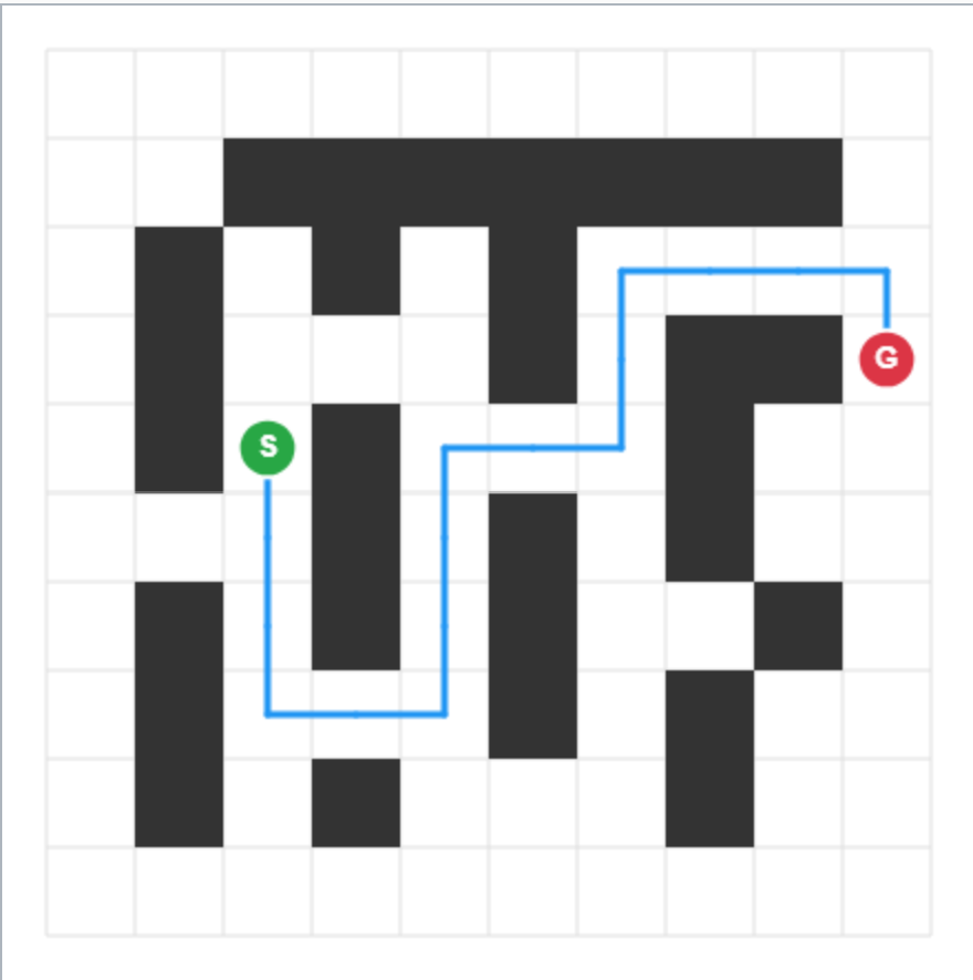
The image displays a 10x10 grid-based maze or pathfinding problem. It features a start point (S), a goal point (G), a series of black obstacle blocks, and a computed blue path connecting the start to the goal while navigating around the obstacles. The diagram visually represents a solution to a spatial navigation problem.
### Components/Axes
* **Grid Structure:** A 10x10 square grid defined by light gray lines. The grid cells are not labeled with coordinates.
* **Start Point (S):** A green circle containing a white letter "S". It is located in the left-center region of the grid.
* **Goal Point (G):** A red circle containing a white letter "G". It is located on the right edge of the grid.
* **Obstacles:** Solid black squares occupying specific grid cells, forming walls and barriers.
* **Path:** A solid blue line tracing a route from the start point to the goal point. The path moves along the edges of the grid cells.
### Detailed Analysis
**Path Trajectory:**
The blue path originates at the center of the green "S" circle. Its route can be described as follows:
1. Moves vertically downward for approximately 2 grid cells.
2. Turns right (east) and moves horizontally for approximately 3 grid cells.
3. Turns upward (north) and moves vertically for approximately 3 grid cells.
4. Turns right (east) and moves horizontally for approximately 2 grid cells.
5. Turns upward (north) and moves vertically for approximately 1 grid cell.
6. Turns right (east) and moves horizontally for approximately 2 grid cells.
7. Turns downward (south) and moves vertically for approximately 1 grid cell, terminating at the center of the red "G" circle.
**Obstacle Layout (Approximate Grid Positions):**
The black obstacles form a complex pattern. Key clusters include:
* A large, inverted "T" shape dominating the top-center.
* Vertical and horizontal bars in the left and central columns.
* Isolated blocks and L-shaped structures in the right-hand columns, creating a narrow corridor the path must navigate through.
### Key Observations
* **Path Efficiency:** The blue path appears to be an optimal or near-optimal route. It takes the shortest possible turns to navigate the maze, suggesting it was generated by a pathfinding algorithm (e.g., A*, Dijkstra's).
* **Spatial Constraints:** The path is forced into a specific, winding route due to the placement of the black obstacles. The most constricted section is in the right-center of the grid, where the path makes a tight "S" curve.
* **Visual Coding:** The diagram uses high-contrast, intuitive colors: green for start (go), red for stop/goal, blue for the solution path, and black for impassable barriers.
### Interpretation
This diagram is a classic representation of a **pathfinding or maze-solving algorithm's output**. It demonstrates the core challenge of navigating from point A to point B in an environment with defined obstacles.
* **What it Suggests:** The image illustrates a successful computational solution to a spatial problem. The blue line is not a random scribble but the result of an algorithm evaluating possible routes and selecting one that minimizes distance or cost while adhering to the constraint of avoiding black cells.
* **Relationship of Elements:** The start (S) and goal (G) define the problem's endpoints. The black obstacles define the problem's constraints or "cost map." The blue line is the solution—the sequence of moves that satisfies the constraints to connect the endpoints.
* **Notable Anomalies:** There are no apparent anomalies in the path itself; it is a logical, continuous line. The maze design is non-trivial, featuring dead ends and a bottleneck, which makes the computed path non-obvious to a human glance, thereby effectively demonstrating the utility of an algorithmic approach.
**In essence, this image is a visual proof-of-concept for an automated navigation system, showing its ability to find a valid route through a complex, structured environment.**