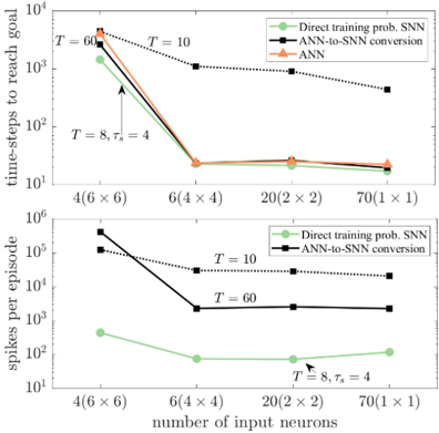
\n ## Line Chart: Performance Comparison of Neural Network Training Methods ### Overview The image contains two vertically stacked line charts comparing the performance of three different methods for training spiking neural networks (SNNs). The charts plot two different performance metrics against the same set of input configurations. The overall purpose is to demonstrate the efficiency and scalability of the "Direct training prob. SNN" method compared to "ANN-to-SNN conversion" and standard "ANN" training. ### Components/Axes **Common Elements (Both Charts):** * **X-Axis (Bottom):** Labeled "number of input neurons". It has four categorical tick marks representing different input layer configurations: * `4(6 x 6)` * `6(4 x 4)` * `20(2 x 2)` * `70(1 x 1)` * **Legend (Top-Right of each chart):** Contains three entries with corresponding line styles and markers: * `Direct training prob. SNN`: Light green line with circular markers. * `ANN-to-SNN conversion`: Black line with square markers. * `ANN`: Orange line with triangular markers. * **Annotations:** Text annotations appear within the plot area, indicating specific parameter settings (`T = 60`, `T = 10`, `T = 8, τ_s = 4`). **Top Chart Specifics:** * **Title/Y-Axis Label:** "time-steps to reach goal". * **Y-Axis Scale:** Logarithmic, ranging from `10^1` to `10^4`. * **Data Series:** All three methods are plotted. **Bottom Chart Specifics:** * **Title/Y-Axis Label:** "spikes per episode". * **Y-Axis Scale:** Logarithmic, ranging from `10^1` to `10^6`. * **Data Series:** Only "Direct training prob. SNN" and "ANN-to-SNN conversion" are plotted. The "ANN" series is absent. ### Detailed Analysis **Top Chart: Time-Steps to Reach Goal** * **Trend Verification:** * **ANN-to-SNN conversion (Black, Squares):** Shows a strong downward trend. Starts highest, decreases sharply, then plateaus. * **ANN (Orange, Triangles):** Follows a very similar downward trend to the ANN-to-SNN line, nearly overlapping it. * **Direct training prob. SNN (Green, Circles):** Also shows a strong downward trend, starting lower than the other two and maintaining a lower value throughout. * **Data Point Extraction (Approximate values from log scale):** * **Input: 4(6x6)** * ANN-to-SNN: ~2000 * ANN: ~2500 * Direct SNN: ~1000 * **Input: 6(4x4)** * ANN-to-SNN: ~20 * ANN: ~20 * Direct SNN: ~15 * **Input: 20(2x2)** * ANN-to-SNN: ~15 * ANN: ~18 * Direct SNN: ~15 * **Input: 70(1x1)** * ANN-to-SNN: ~15 * ANN: ~18 * Direct SNN: ~15 * **Annotations:** * `T = 60` points to the first data point of the ANN-to-SNN line. * `T = 10` points to the first data point of the ANN line. * `T = 8, τ_s = 4` points to the first data point of the Direct SNN line. **Bottom Chart: Spikes per Episode** * **Trend Verification:** * **ANN-to-SNN conversion (Black, Squares):** Shows a strong downward trend, then plateaus. Two distinct lines are visible for this series, labeled `T = 10` (higher) and `T = 60` (lower). * **Direct training prob. SNN (Green, Circles):** Shows a moderate downward trend, then a slight upward trend at the end. It is consistently orders of magnitude lower than the ANN-to-SNN method. * **Data Point Extraction (Approximate values from log scale):** * **Input: 4(6x6)** * ANN-to-SNN (T=10): ~200,000 * ANN-to-SNN (T=60): ~40,000 * Direct SNN: ~400 * **Input: 6(4x4)** * ANN-to-SNN (T=10): ~30,000 * ANN-to-SNN (T=60): ~2,000 * Direct SNN: ~60 * **Input: 20(2x2)** * ANN-to-SNN (T=10): ~20,000 * ANN-to-SNN (T=60): ~2,000 * Direct SNN: ~60 * **Input: 70(1x1)** * ANN-to-SNN (T=10): ~20,000 * ANN-to-SNN (T=60): ~2,000 * Direct SNN: ~100 * **Annotations:** * `T = 10` and `T = 60` label the two black lines for the ANN-to-SNN method. * `T = 8, τ_s = 4` points to the first data point of the Direct SNN line. ### Key Observations 1. **Performance Convergence:** For the "time-steps to reach goal" metric, all three methods converge to very similar, low values (~15-20 time-steps) as the number of input neurons increases (moving right on the x-axis). The initial advantage of the Direct SNN method diminishes. 2. **Massive Efficiency Gap:** The most striking observation is in the "spikes per episode" chart. The Direct training SNN method uses **3 to 4 orders of magnitude fewer spikes** than the ANN-to-SNN conversion method across all input configurations. This indicates vastly superior energy efficiency for the direct training approach. 3. **Impact of Parameter T:** For the ANN-to-SNN conversion method, a higher `T` value (60 vs. 10) results in significantly fewer spikes per episode (by about an order of magnitude), while having a negligible effect on the time-steps to reach the goal in the top chart. 4. **Scalability:** The Direct SNN method shows relatively stable and low spike counts as the input configuration changes, suggesting good scalability. The ANN-to-SNN method's spike count also stabilizes but at a much higher level. ### Interpretation This data presents a compelling case for the "Direct training prob. SNN" method. While all methods can solve the task in a similar number of time-steps once the input is sufficiently high-dimensional, the **computational cost** (measured in spikes, a proxy for energy consumption in neuromorphic hardware) is dramatically different. The charts suggest that traditional ANN-to-SNN conversion methods incur a massive overhead in spiking activity. The direct training approach successfully optimizes the SNN to perform the task with minimal spiking, which is the core advantage of SNNs. The parameter `T` (likely representing simulation time-steps or a time constant) is a critical tuning knob for the conversion method, trading off between spike efficiency and potentially other factors not shown here. **Conclusion:** The visualization argues that for building efficient, low-power spiking neural networks, directly training the SNN with a probabilistic framework is vastly superior to converting a pre-trained ANN, especially when the primary metric is energy efficiency (spike count). The task performance (time-steps) becomes comparable with sufficient input complexity.