\n
## Line Chart: Accuracy vs. Number of Samples for Think@n and Cons@n
### Overview
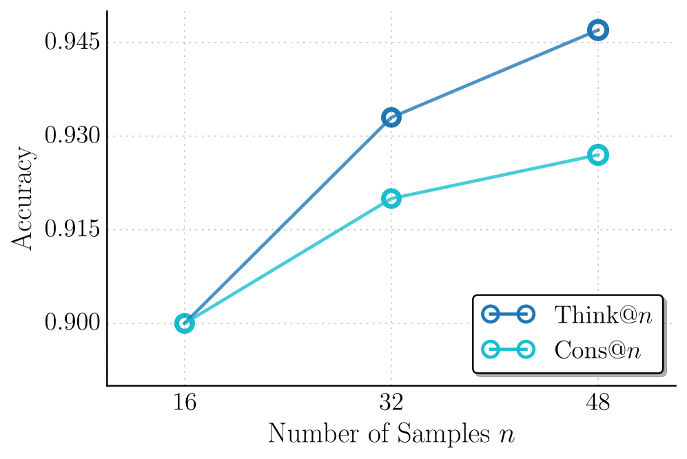
The image is a line chart comparing the performance (accuracy) of two methods, labeled "Think@n" and "Cons@n", as the number of samples (`n`) increases. The chart demonstrates that both methods improve with more samples, but "Think@n" shows a greater rate of improvement.
### Components/Axes
* **X-Axis (Horizontal):** Labeled "Number of Samples `n`". It has three discrete, evenly spaced tick marks at values 16, 32, and 48.
* **Y-Axis (Vertical):** Labeled "Accuracy". The scale is linear, with labeled tick marks at 0.900, 0.915, 0.930, and 0.945. The axis extends slightly below 0.900 and above 0.945.
* **Legend:** Located in the bottom-right corner of the plot area, enclosed in a box. It contains two entries:
* A dark blue line with circle markers labeled `Think@n`.
* A light blue (cyan) line with circle markers labeled `Cons@n`.
* **Grid:** A faint, dotted grid is present in the background, aligned with the major tick marks on both axes.
### Detailed Analysis
**Data Series: Think@n (Dark Blue Line)**
* **Trend:** The line slopes steeply upward from left to right, indicating a strong positive correlation between sample size and accuracy.
* **Data Points (Approximate):**
* At `n = 16`: Accuracy ≈ 0.900
* At `n = 32`: Accuracy ≈ 0.932
* At `n = 48`: Accuracy ≈ 0.946
**Data Series: Cons@n (Light Blue Line)**
* **Trend:** The line also slopes upward, but with a less steep gradient compared to the Think@n line, indicating a positive but more moderate improvement.
* **Data Points (Approximate):**
* At `n = 16`: Accuracy ≈ 0.900 (appears to start at the same point as Think@n)
* At `n = 32`: Accuracy ≈ 0.920
* At `n = 48`: Accuracy ≈ 0.927
### Key Observations
1. **Common Starting Point:** Both methods begin at approximately the same accuracy (0.900) when the number of samples is 16.
2. **Diverging Performance:** As the number of samples increases to 32 and 48, the performance of the two methods diverges. The gap in accuracy between Think@n and Cons@n widens with larger `n`.
3. **Superior Scaling of Think@n:** The Think@n method demonstrates superior scalability, achieving a higher final accuracy (≈0.946 vs. ≈0.927) and a greater overall gain (≈0.046 vs. ≈0.027) over the tested range.
4. **Diminishing Returns for Cons@n:** The slope of the Cons@n line appears to flatten slightly between `n=32` and `n=48`, suggesting potential diminishing returns, whereas the Think@n line maintains a strong upward trajectory.
### Interpretation
The chart presents a comparative analysis of two algorithmic or procedural methods ("Think@n" and "Cons@n") in a machine learning or statistical context, where performance is measured by accuracy on a task.
* **What the data suggests:** The data strongly suggests that the "Think@n" method is more effective at leveraging additional data samples to improve its accuracy. While both methods benefit from more data, "Think@n" has a higher "learning efficiency" or better model capacity within this sample size regime.
* **Relationship between elements:** The x-axis (input resource: samples) is the independent variable, and the y-axis (output quality: accuracy) is the dependent variable. The two lines represent different models or strategies for converting the input resource into output quality. The widening gap indicates that the choice of method becomes increasingly consequential as more data becomes available.
* **Notable implications:** For a practitioner, this chart argues for adopting the "Think@n" approach if the goal is to maximize accuracy and if a sample size of 32 or more is available. The "Cons@n" method might be preferable only under constraints where `n` is very small (≤16) or if it offers significant advantages not shown here (e.g., lower computational cost, faster inference). The chart does not show performance for `n < 16` or `n > 48`, so conclusions are limited to this range.