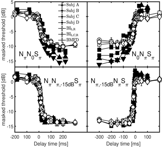
## Chart: Masked Threshold vs. Delay Time ### Overview The image presents two plots displaying masked threshold [dB] as a function of delay time [ms]. The plots appear to represent psychoacoustic data, likely from auditory experiments. Each plot shows data for multiple subjects and a model (BMED). The top plot shows data for a 0 dB signal-to-noise ratio, while the bottom plot shows data for a -15 dB signal-to-noise ratio. ### Components/Axes * **X-axis (both plots):** Delay time [ms]. Scale ranges from -200 ms to 200 ms in the top plot and -300 ms to 100 ms in the bottom plot. * **Y-axis (both plots):** Masked threshold [dB]. Scale ranges from -15 dB to 5 dB. * **Legend (top-right):** * Subj A (Black squares) * Subj B (Black circles) * Subj C (Black triangles pointing up) * Subj D (Black diamonds) * BIL_R (Gray squares) * BIL_C,R (Gray circles) * BMED (Black squares) * **Labels (top plot):** N N S_π, N₀ S_π * **Labels (bottom plot):** N N_π,-15dB S_π, N_π,-15dB N S_π ### Detailed Analysis or Content Details **Top Plot (0 dB SNR):** * **Subj A (Black squares):** The line slopes downward from approximately 2 dB at -200 ms to approximately -14 dB at 150 ms, then rises again to approximately -8 dB at 200 ms. * Approximate data points: (-200, 2), (-100, -6), (0, -10), (100, -14), (200, -8) * **Subj B (Black circles):** The line slopes downward from approximately 1 dB at -200 ms to approximately -13 dB at 150 ms, then rises again to approximately -7 dB at 200 ms. * Approximate data points: (-200, 1), (-100, -5), (0, -9), (100, -13), (200, -7) * **Subj C (Black triangles):** The line slopes downward from approximately 0 dB at -200 ms to approximately -12 dB at 150 ms, then rises again to approximately -6 dB at 200 ms. * Approximate data points: (-200, 0), (-100, -4), (0, -8), (100, -12), (200, -6) * **Subj D (Black diamonds):** The line slopes downward from approximately 1 dB at -200 ms to approximately -15 dB at 150 ms, then rises again to approximately -9 dB at 200 ms. * Approximate data points: (-200, 1), (-100, -6), (0, -11), (100, -15), (200, -9) * **BIL_R (Gray squares):** The line slopes downward from approximately 0 dB at -200 ms to approximately -10 dB at 150 ms, then rises again to approximately -5 dB at 200 ms. * Approximate data points: (-200, 0), (-100, -4), (0, -7), (100, -10), (200, -5) * **BIL_C,R (Gray circles):** The line slopes downward from approximately 0 dB at -200 ms to approximately -9 dB at 150 ms, then rises again to approximately -4 dB at 200 ms. * Approximate data points: (-200, 0), (-100, -3), (0, -6), (100, -9), (200, -4) * **BMED (Black squares):** The line slopes downward from approximately 0 dB at -200 ms to approximately -12 dB at 150 ms, then rises again to approximately -7 dB at 200 ms. * Approximate data points: (-200, 0), (-100, -5), (0, -9), (100, -12), (200, -7) **Bottom Plot (-15 dB SNR):** * **Subj A (Black squares):** The line remains relatively flat around -1 dB to -2 dB from -300 ms to 0 ms, then rises to approximately 0 dB at 100 ms. * Approximate data points: (-300, -1), (-200, -1), (-100, -2), (0, -2), (100, 0) * **Subj B (Black circles):** The line remains relatively flat around -1 dB to -2 dB from -300 ms to 0 ms, then rises to approximately 0 dB at 100 ms. * Approximate data points: (-300, -1), (-200, -1), (-100, -2), (0, -2), (100, 0) * **Subj C (Black triangles):** The line remains relatively flat around -1 dB to -2 dB from -300 ms to 0 ms, then rises to approximately 0 dB at 100 ms. * Approximate data points: (-300, -1), (-200, -1), (-100, -2), (0, -2), (100, 0) * **Subj D (Black diamonds):** The line remains relatively flat around -1 dB to -2 dB from -300 ms to 0 ms, then rises to approximately 0 dB at 100 ms. * Approximate data points: (-300, -1), (-200, -1), (-100, -2), (0, -2), (100, 0) * **BIL_R (Gray squares):** The line remains relatively flat around -1 dB to -2 dB from -300 ms to 0 ms, then rises to approximately 0 dB at 100 ms. * Approximate data points: (-300, -1), (-200, -1), (-100, -2), (0, -2), (100, 0) * **BIL_C,R (Gray circles):** The line remains relatively flat around -1 dB to -2 dB from -300 ms to 0 ms, then rises to approximately 0 dB at 100 ms. * Approximate data points: (-300, -1), (-200, -1), (-100, -2), (0, -2), (100, 0) * **BMED (Black squares):** The line remains relatively flat around -1 dB to -2 dB from -300 ms to 0 ms, then rises to approximately 0 dB at 100 ms. * Approximate data points: (-300, -1), (-200, -1), (-100, -2), (0, -2), (100, 0) ### Key Observations * In the top plot (0 dB SNR), all curves exhibit a U-shaped pattern, indicating a minimum in masked threshold at around 100-150 ms delay. * In the bottom plot (-15 dB SNR), the curves are much flatter, suggesting that the masked threshold is less sensitive to delay time at this lower SNR. * The individual subject data (Subj A, B, C, D) generally follows similar trends, with some variability. * The BMED model appears to align well with the average trend of the subject data. * The BIL models (BIL_R and BIL_C,R) show slightly different responses compared to the individual subjects and BMED. ### Interpretation The data suggests that the masking effect of a tone is dependent on the delay between the tone and the masker. At a 0 dB SNR, there is a clear temporal window where masking is most effective (around 100-150 ms delay). This is likely due to the interaction of the signals in the auditory system, potentially related to temporal integration or forward masking. At a -15 dB SNR, the masking effect is less pronounced, and the masked threshold is less sensitive to delay time. This is expected, as the weaker signal is more easily masked regardless of the delay. The BMED model provides a reasonable approximation of the observed data, suggesting that it captures some of the key mechanisms underlying masking. The differences between the BIL models and the subject data may indicate that these models do not fully account for the complexity of human auditory processing. The labels N N S_π, N₀ S_π, N N_π,-15dB S_π, N_π,-15dB N S_π likely refer to the conditions of the experiment, potentially related to the type of signal (N) and masker (S) and their relative phases (π). Further context about the experimental setup would be needed to fully interpret these labels.