## Scatter Plot: MA vs. C
### Overview
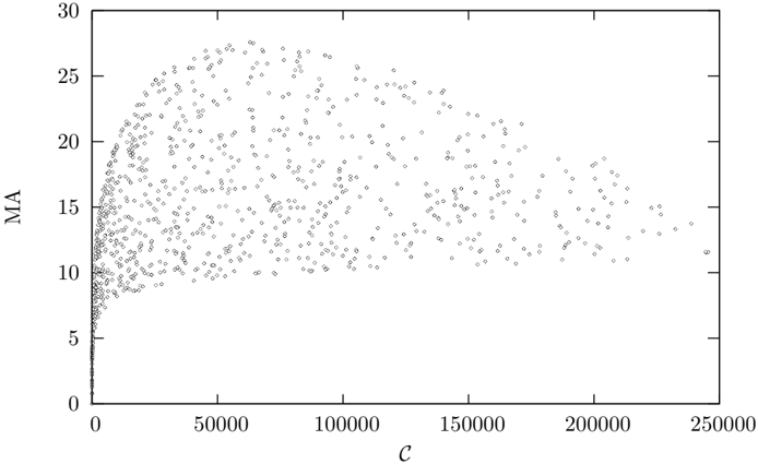
The image displays a scatter plot showing the relationship between two variables, labeled "C" on the horizontal axis and "MA" on the vertical axis. The plot contains a large number of data points (several hundred to a few thousand), all rendered as small, gray, open circles. The data shows a dense concentration near the origin that spreads out significantly as the value of C increases.
### Components/Axes
* **Chart Type:** Scatter Plot.
* **X-Axis:**
* **Label:** `C` (italicized).
* **Scale:** Linear.
* **Range:** 0 to 250,000.
* **Major Tick Marks & Labels:** 0, 50000, 100000, 150000, 200000, 250000.
* **Y-Axis:**
* **Label:** `MA` (italicized).
* **Scale:** Linear.
* **Range:** 0 to 30.
* **Major Tick Marks & Labels:** 0, 5, 10, 15, 20, 25, 30.
* **Legend:** None present. All data points are represented by the same symbol and color (gray circles).
* **Data Points:** Represented as small, gray, open circles. No other distinguishing features (e.g., color, shape) are used to categorize the data.
### Detailed Analysis
* **Data Distribution & Density:**
* The highest density of points is concentrated in the region where `C` is between 0 and approximately 25,000, and `MA` is between 0 and 15.
* As `C` increases beyond 25,000, the points become more dispersed, covering a wider range of `MA` values.
* **Trend Description (Visual):** The overall cloud of points suggests a positive, but highly variable, relationship. The lower boundary of the point cloud appears to slope upward from the origin. The upper boundary also shows an upward trend, but with much greater scatter. The vertical spread (variance in `MA`) for a given `C` increases substantially as `C` increases.
* **Approximate Data Ranges:**
* For `C` < 10,000: `MA` values range from near 0 up to ~20.
* For `C` between 50,000 and 100,000: `MA` values are spread roughly between 8 and 28.
* For `C` > 150,000: The number of points decreases, but they are scattered widely, with `MA` values ranging from approximately 10 to 20. The maximum observed `MA` appears to decrease slightly for the highest `C` values (above 200,000).
### Key Observations
1. **Heteroscedasticity:** The variance of `MA` is not constant across values of `C`. The spread of `MA` values increases dramatically as `C` increases, indicating a strong heteroscedastic relationship.
2. **Density Gradient:** The data is extremely dense near the origin (`C` and `MA` both low) and becomes progressively sparser towards the top-right of the plot.
3. **Potential Ceiling Effect:** There appears to be an upper bound or ceiling for `MA` around the value of 30, with very few points approaching this limit, and none exceeding it.
4. **Sparse High-C Region:** Data points with `C` values above 200,000 are relatively rare compared to the lower `C` regions.
### Interpretation
The scatter plot demonstrates a positive but noisy association between the variables `C` and `MA`. The key insight is not a simple linear correlation, but the structure of the variance.
* **Relationship:** Higher values of `C` are generally associated with higher possible values of `MA`, but also with much greater uncertainty or variability in `MA`. A low `C` value reliably predicts a low-to-moderate `MA`, while a high `C` value could correspond to a wide range of `MA` outcomes.
* **Underlying Phenomenon:** This pattern is characteristic of processes where the factor represented by `C` enables or scales the potential for `MA`, but other, unmeasured factors become increasingly influential as `C` grows. For example, `C` could be "computational resources" and `MA` "model accuracy," where more resources allow for higher accuracy but also introduce more variables (like algorithm choice, data quality) that cause greater spread in results.
* **Data Quality/Collection:** The extreme density at low values suggests either a natural clustering of observations in that regime or a sampling bias where low-`C` scenarios are more frequently observed or measured. The sparsity at high `C` may indicate these conditions are rarer, more expensive to generate, or harder to measure.
* **Investigative Focus:** An analyst should investigate the causes of the increasing variance. The points forming the upper edge of the cloud might represent optimal conditions or efficient processes, while those on the lower edge might indicate inefficiencies or confounding negative factors. The plot argues against using a simple linear model without also modeling the variance structure (e.g., using weighted regression or a generalized linear model).