## Line Graphs: Gibbs Error vs Generalisation Error Across Dimensionality
### Overview
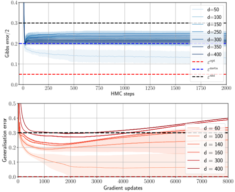
The image contains two vertically stacked line graphs comparing error metrics across different dimensionalities (d). The top graph tracks Gibbs error (normalized by 2) over Hamiltonian Monte Carlo (HMC) steps, while the bottom graph tracks generalization error over gradient updates. Both graphs include multiple data series for varying dimensionalities and reference lines for theoretical error bounds.
### Components/Axes
**Top Graph (Gibbs Error):**
- **X-axis**: HMC steps (0–2000, linear scale)
- **Y-axis**: Gibbs error / 2 (0–0.4, linear scale)
- **Legend**:
- Solid lines: d=50 (light blue), d=100 (medium blue), d=150 (dark blue), d=250 (navy), d=300 (dark blue), d=350 (navy), d=400 (black)
- Dashed lines: ε_opt (red), ε_meta (blue), ε_uni (black)
- **Key markers**: Vertical dashed line at HMC step 50
**Bottom Graph (Generalisation Error):**
- **X-axis**: Gradient updates (0–8000, linear scale)
- **Y-axis**: Generalisation error (0–0.5, linear scale)
- **Legend**:
- Solid lines: d=60 (light orange), d=100 (orange), d=140 (dark orange), d=160 (red), d=300 (maroon), d=400 (dark red)
- **Key markers**: Horizontal dashed line at y=0.3
### Detailed Analysis
**Top Graph Trends:**
1. All d values show an initial sharp decline in Gibbs error within the first 50 HMC steps, dropping from ~0.35 to ~0.2.
2. Post-50 steps, all d values converge to a stable error band between 0.2–0.25, with minimal variation.
3. Theoretical bounds:
- ε_opt (red dashed): ~0.15
- ε_meta (blue dashed): ~0.2
- ε_uni (black dashed): ~0.3
4. d=400 (black line) shows the fastest convergence but remains slightly above ε_meta.
**Bottom Graph Trends:**
1. Lower d values (d=60–160) start with higher errors (~0.45–0.5) but decrease sharply within 1000 updates to ~0.25–0.3.
2. Higher d values (d=300–400) begin with lower errors (~0.3–0.35) but show a gradual increase after 5000 updates, reaching ~0.4–0.45 by 8000 updates.
3. All lines exhibit increasing variance (shaded regions) as gradient updates progress.
### Key Observations
1. **Top Graph**:
- Gibbs error stabilizes rapidly (<50 steps) and becomes insensitive to d.
- ε_meta (blue dashed) acts as a practical upper bound for most d values.
- d=400 approaches ε_opt (red dashed) more closely than other d values.
2. **Bottom Graph**:
- Lower d values show better generalization initially but risk overfitting at higher updates.
- Higher d values demonstrate worse generalization over time, suggesting potential overfitting.
- d=100 and d=140 show the most stable generalization performance.
### Interpretation
The top graph reveals that Gibbs error convergence is largely dimension-agnostic after initial optimization, with theoretical bounds (ε_meta/ε_opt) providing meaningful reference points. The bottom graph highlights a trade-off between dimensionality and generalization: lower d values achieve better generalization initially but may overfit with prolonged training, while higher d values start stronger but degrade performance. This suggests careful dimensionality selection is critical – too low risks underfitting, too high risks overfitting. The convergence patterns imply that HMC steps are more critical for initial error reduction than gradient updates for generalization stability.