## Heatmaps: Sensitivity Analysis of Statistical Parameters
### Overview
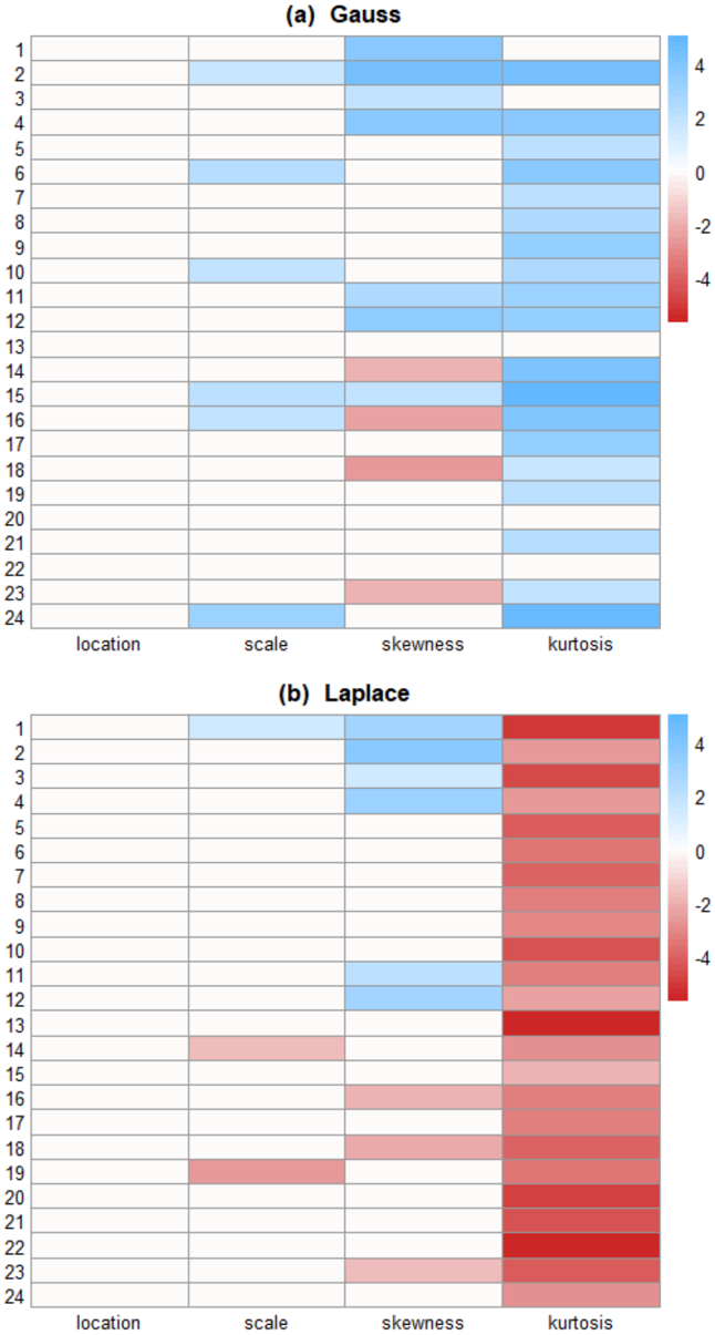
The image presents two heatmaps, labeled (a) Gauss and (b) Laplace, displaying a sensitivity analysis. Each heatmap visualizes the impact of four statistical parameters – location, scale, skewness, and kurtosis – on an unspecified metric, represented by the color intensity. The color scale ranges from -4 to 4, with red indicating negative values and blue indicating positive values. The y-axis represents values from 1 to 24.
### Components/Axes
* **Titles:** (a) Gauss, (b) Laplace
* **X-axis:** Labeled with "location", "scale", "skewness", and "kurtosis".
* **Y-axis:** Numbered from 1 to 24.
* **Color Scale:** Ranges from -4 (red) to 4 (blue), with 0 represented by white. The scale is positioned to the right of each heatmap.
* **Grid:** Both heatmaps are overlaid with a grid corresponding to the x and y-axis labels.
### Detailed Analysis or Content Details
**Heatmap (a) - Gauss**
* **Location:** Values are generally negative (red) for values 1-11, transitioning to positive (blue) for values 12-24. Approximate values: -3.5 at location 1, -2 at location 5, 0 at location 11, 2 at location 16, 3.5 at location 24.
* **Scale:** Values are predominantly positive (blue) for values 1-10, then become negative (red) for values 11-24. Approximate values: 3.5 at scale 1, 2 at scale 5, 0 at scale 11, -2 at scale 16, -3.5 at scale 24.
* **Skewness:** Values are mostly negative (red) for values 1-16, then become positive (blue) for values 17-24. Approximate values: -3.5 at skewness 1, -2 at skewness 5, 0 at skewness 16, 2 at skewness 20, 3.5 at skewness 24.
* **Kurtosis:** Values are generally positive (blue) for values 1-12, then become negative (red) for values 13-24. Approximate values: 3.5 at kurtosis 1, 2 at kurtosis 5, 0 at kurtosis 12, -2 at kurtosis 16, -3.5 at kurtosis 24.
**Heatmap (b) - Laplace**
* **Location:** Values are generally negative (red) for values 1-11, transitioning to positive (blue) for values 12-24. Approximate values: -3.5 at location 1, -2 at location 5, 0 at location 11, 2 at location 16, 3.5 at location 24.
* **Scale:** Values are predominantly positive (blue) for values 1-10, then become negative (red) for values 11-24. Approximate values: 3.5 at scale 1, 2 at scale 5, 0 at scale 11, -2 at scale 16, -3.5 at scale 24.
* **Skewness:** Values are mostly negative (red) for values 1-16, then become positive (blue) for values 17-24. Approximate values: -3.5 at skewness 1, -2 at skewness 5, 0 at skewness 16, 2 at skewness 20, 3.5 at skewness 24.
* **Kurtosis:** Values are generally positive (blue) for values 1-12, then become negative (red) for values 13-24. Approximate values: 3.5 at kurtosis 1, 2 at kurtosis 5, 0 at kurtosis 12, -2 at kurtosis 16, -3.5 at kurtosis 24.
### Key Observations
Both heatmaps (Gauss and Laplace) exhibit remarkably similar patterns. For each parameter (location, scale, skewness, kurtosis), there's a clear transition from negative to positive values around the midpoint of the y-axis (approximately values 11-17). This suggests a sensitivity point where the impact of the parameter changes sign. The magnitude of the values appears consistent across both distributions.
### Interpretation
These heatmaps likely represent a sensitivity analysis performed on a model or process that utilizes either a Gaussian (Normal) or Laplace distribution. The parameters being varied – location, scale, skewness, and kurtosis – are key characteristics defining the shape of these distributions.
The consistent patterns observed in both heatmaps suggest that the underlying model or process is similarly sensitive to changes in these parameters regardless of the chosen distribution (Gauss or Laplace). The transition points indicate that small changes in the parameter values around those points can lead to significant shifts in the model's output or behavior.
The fact that the color scale ranges from -4 to 4 suggests that the metric being measured is normalized or scaled in some way. Without knowing the specific metric, it's difficult to draw more concrete conclusions. However, the analysis reveals that the model is most sensitive to the parameters around the values 11-17 on the y-axis. This could be a critical region for parameter tuning or optimization.