TECHNICAL ASSET FINGERPRINT
8ba867dab0359323dbf93adc
Click to view fullscreen
Press ESC or click to close
FOUND IN PAPERS
EXPERT: healer-alpha-free VERSION 1
RUNTIME: free/openrouter/healer-alpha
INTEL_VERIFIED
\n
## [Multi-Panel Chart]: Comparison of Process Reward Models (PRMs) and Prover Performance
### Overview
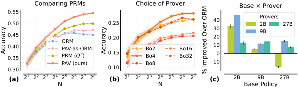
The image contains three distinct subplots labeled (a), (b), and (c), presenting a comparative analysis of different Process Reward Models (PRMs) and "Prover" configurations in a machine learning context. The charts evaluate performance based on accuracy and percentage improvement over a baseline model (ORM).
### Components/Axes
**General Layout:** Three charts arranged horizontally. Each has its own title, axes, and legend.
**Subplot (a): "Comparing PRMs"**
* **Type:** Line chart with shaded confidence intervals.
* **X-axis:** Label: "N". Scale: Logarithmic base 2, with markers at 2¹, 2², 2³, 2⁴, 2⁵, 2⁶, 2⁷, 2⁸.
* **Y-axis:** Label: "Accuracy". Scale: Linear, from 0.30 to 0.55 in increments of 0.05.
* **Legend:** Positioned in the bottom-right quadrant. Contains four entries:
* `ORM` (Blue, dashed line with circle markers)
* `PAV-as-ORM` (Pink, dashed line with circle markers)
* `PRM (Q^π)` (Olive green, dashed line with circle markers)
* `PAV (ours)` (Orange, solid line with circle markers)
**Subplot (b): "Choice of Prover"**
* **Type:** Line chart with shaded confidence intervals.
* **X-axis:** Label: "N". Scale: Logarithmic base 2, with markers at 2¹, 2², 2³, 2⁴, 2⁵, 2⁶, 2⁷.
* **Y-axis:** Label: "Accuracy". Scale: Linear, from 0.10 to 0.25 in increments of 0.05.
* **Legend:** Positioned in the bottom-right quadrant. Contains five entries:
* `Bo2` (Orange, dashed line with circle markers)
* `Bo4` (Brown, solid line with circle markers)
* `Bo8` (Dark orange, dashed line with circle markers)
* `Bo16` (Light orange, dashed line with circle markers)
* `Bo32` (Red, dashed line with circle markers)
**Subplot (c): "Base x Prover"**
* **Type:** Grouped bar chart with error bars.
* **X-axis:** Label: "Base Policy". Categories: `2B`, `9B`, `27B`.
* **Y-axis:** Label: "% Improved Over ORM". Scale: Linear, from -10 to 40 in increments of 10.
* **Legend:** Positioned in the top-right quadrant. Title: "Provers". Contains three entries:
* `2B` (Yellow-green bar)
* `9B` (Blue bar)
* `27B` (Teal bar)
### Detailed Analysis
**Subplot (a) Analysis:**
* **Trend Verification:** All four lines show an upward trend as N increases, indicating improving accuracy with larger N. The `PAV (ours)` line has the steepest and most consistent upward slope.
* **Data Points (Approximate):**
* At N=2¹: All models start near 0.32-0.33 accuracy.
* At N=2⁴: `ORM` ~0.44, `PAV-as-ORM` ~0.45, `PRM (Q^π)` ~0.46, `PAV (ours)` ~0.48.
* At N=2⁸: `ORM` ~0.46, `PAV-as-ORM` ~0.47, `PRM (Q^π)` ~0.50, `PAV (ours)` ~0.55.
* **Key Observation:** The proposed method `PAV (ours)` consistently outperforms the other three methods across all values of N, with the performance gap widening as N increases.
**Subplot (b) Analysis:**
* **Trend Verification:** All lines show an upward trend with increasing N. The lines for `Bo2`, `Bo4`, and `Bo8` are tightly clustered and show the strongest improvement. `Bo16` and `Bo32` show lower accuracy and a shallower slope.
* **Data Points (Approximate):**
* At N=2¹: All models start between 0.11 and 0.15.
* At N=2⁷: `Bo2` ~0.26, `Bo4` ~0.27, `Bo8` ~0.26, `Bo16` ~0.22, `Bo32` ~0.21.
* **Key Observation:** Smaller "Bo" values (2, 4, 8) lead to significantly higher final accuracy compared to larger values (16, 32). `Bo4` appears to achieve the highest peak accuracy.
**Subplot (c) Analysis:**
* **Spatial Grounding:** For each "Base Policy" category on the x-axis, three bars are grouped, corresponding to the "Prover" sizes in the legend (2B, 9B, 27B).
* **Data Points (Approximate % Improvement):**
* **Base Policy 2B:** Prover 2B: ~32%, Prover 9B: ~45% (highest bar in chart), Prover 27B: ~13%.
* **Base Policy 9B:** Prover 2B: ~5%, Prover 9B: ~12%, Prover 27B: ~15%.
* **Base Policy 27B:** Prover 2B: ~-12% (negative improvement), Prover 9B: ~15%, Prover 27B: ~8%.
* **Key Observation:** The combination of a small base policy (2B) with a medium-sized prover (9B) yields the greatest improvement over ORM. Using a prover much larger than the base policy (e.g., 27B prover with 2B base) is less effective. Notably, using a 2B prover with a 27B base policy results in performance *worse* than the ORM baseline.
### Key Observations
1. **Dominant Method:** In subplot (a), `PAV (ours)` is the clear top performer, suggesting it is the most effective PRM variant tested.
2. **Optimal Prover Size:** Subplot (b) indicates that moderate "Bo" values (2-8) are optimal for accuracy, while larger values (16, 32) degrade performance.
3. **Critical Interaction:** Subplot (c) reveals a crucial interaction between base policy size and prover size. Performance is not simply "bigger is better." The most significant gains come from pairing a small base with a moderately larger prover. The negative result for (27B Base, 2B Prover) is a critical outlier.
4. **Scaling Trend:** Both line charts (a & b) demonstrate that accuracy improves with the parameter N, but the rate of improvement and ceiling differ by method.
### Interpretation
This set of charts likely comes from research on improving the reasoning or verification capabilities of language models using process-based reward models. The data suggests several key findings:
1. **Superiority of PAV:** The proposed "PAV" method (subplot a) is more effective at leveraging increased computational resources (N) to improve accuracy compared to existing methods like ORM and standard PRMs. This indicates a more efficient or accurate reward modeling approach.
2. **Importance of Prover Calibration:** The "Choice of Prover" (subplot b) shows that the prover's own configuration (the "Bo" parameter, possibly related to beam search width or branching factor) is a critical hyperparameter. There's a sweet spot; an overly broad or narrow search (high or low Bo) is suboptimal. This implies the prover must be carefully tuned to match the difficulty of the task or the capability of the reward model.
3. **The Base-Prover Synergy:** The most insightful finding is in subplot (c). It demonstrates that the effectiveness of a prover is highly dependent on the size/capability of the base policy it is augmenting. The dramatic improvement for the 2B base with a 9B prover suggests a synergistic effect where a capable prover can significantly boost a weaker base model. Conversely, a weak prover (2B) cannot help, and may even hinder, a strong base model (27B), possibly by introducing noise or incorrect guidance. This highlights the need for balanced system design rather than independently scaling components.
**Overall, the investigation argues for the adoption of the PAV method and emphasizes that optimal system performance requires co-design and careful balancing of the base policy model size and the prover's search configuration.**
DECODING INTELLIGENCE...