## Diagram: Optimization Paths for Different Penalty Methods in Multi-Task Learning
### Overview
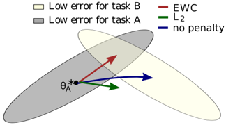
The image is a conceptual diagram illustrating the optimization trajectories of three different penalty (regularization) methods when moving from a solution optimal for one task (Task A) towards a region that is also good for a second task (Task B). It visually compares how Elastic Weight Consolidation (EWC), L2 regularization, and no penalty affect the parameter update direction.
### Components/Axes
* **Legend (Top Center):**
* **Light Yellow Rectangle:** "Low error for task B"
* **Gray Rectangle:** "Low error for task A"
* **Red Line:** "EWC"
* **Green Line:** "L2"
* **Blue Line:** "no penalty"
* **Key Elements in Diagram:**
* **Gray Ellipse:** Represents the region of parameter space where Task A has low error. It is oriented diagonally from lower-left to upper-right.
* **Light Yellow Ellipse:** Represents the region of parameter space where Task B has low error. It is also oriented diagonally but is shifted to the right and slightly upward relative to the gray ellipse, creating an overlapping region.
* **Point θ_A*:** A black dot located in the lower-left portion of the gray ellipse, representing the optimal parameter set for Task A alone.
* **Arrows (Vectors):** Three colored arrows originate from θ_A*, indicating the direction of parameter update suggested by each method.
* **Red Arrow (EWC):** Points diagonally upward and to the right, directly into the overlapping region of the two ellipses.
* **Green Arrow (L2):** Points to the right and slightly downward, towards the center of the gray (Task A) ellipse.
* **Blue Arrow (no penalty):** Points directly to the right, towards the center of the light yellow (Task B) ellipse.
### Detailed Analysis
The diagram is a qualitative, not quantitative, representation. It shows the **directional intent** of each optimization method starting from θ_A*.
* **Spatial Relationships:** The two ellipses overlap in the upper-center area of the diagram. The point θ_A* is situated well within the gray (Task A) ellipse but outside the light yellow (Task B) ellipse.
* **Trend Verification (Directional Vectors):**
* **EWC (Red):** The vector slopes upward, aiming for the compromise region where both tasks have low error. This suggests EWC seeks a solution that retains performance on Task A while improving on Task B.
* **L2 (Green):** The vector has a shallow downward slope, pulling the parameters back towards the center of the original task's (Task A) low-error region. This suggests L2 regularization primarily constrains the solution to stay near the original task's optimum.
* **No Penalty (Blue):** The vector is horizontal, moving directly towards the center of the new task's (Task B) low-error region. This suggests that without a penalty, optimization would fully shift to minimize error on Task B, potentially at the expense of Task A.
### Key Observations
1. **Divergent Goals:** The three methods produce distinctly different update directions from the same starting point (θ_A*).
2. **EWC as a Compromise:** The EWC path is the only one that points directly into the intersection of the two low-error regions, visually representing its goal of finding a shared solution.
3. **L2 as an Anchor:** The L2 path is "anchored" towards the original task's solution space, indicating it acts as a conservative regularizer.
4. **No Penalty as a Full Shift:** The "no penalty" path shows a complete directional shift towards the new task, illustrating the problem of catastrophic forgetting where learning a new task can overwrite knowledge of the old one.
### Interpretation
This diagram is a pedagogical tool explaining the core intuition behind **continual learning** or **multi-task learning** regularization techniques.
* **What it demonstrates:** It visually argues that different regularization methods encode different *inductive biases* about how to navigate the loss landscape when faced with a new task. The choice of method fundamentally changes the optimization trajectory.
* **Relationship between elements:** The ellipses define the "solution spaces" for individual tasks. The arrows represent the "policy" of each algorithm. The starting point θ_A* represents the model's state after learning the first task. The diagram's central message is that the policy (penalty method) determines whether the model moves towards a compromise (EWC), stays anchored to the past (L2), or fully commits to the new task (no penalty).
* **Underlying Message:** The diagram implicitly advocates for methods like EWC that explicitly model and protect important parameters for previous tasks (represented by the direction towards the overlap), as opposed to naive fine-tuning (no penalty) or simple weight decay (L2), which may not effectively balance multiple tasks. It highlights the geometric challenge of finding parameters that lie in the intersection of multiple, potentially misaligned, low-error regions.