TECHNICAL ASSET FINGERPRINT
8c5e56a17702a9457b724a0e
Click to view fullscreen
Press ESC or click to close
FOUND IN PAPERS
EXPERT: healer-alpha-free VERSION 1
RUNTIME: free/openrouter/healer-alpha
INTEL_VERIFIED
\n
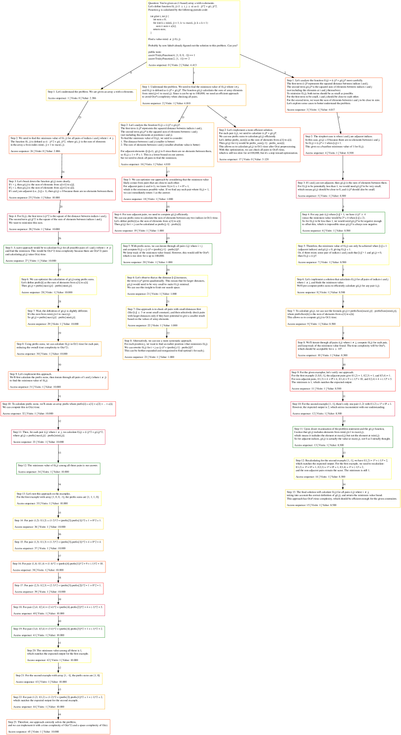
## Flowchart/Diagram: Algorithmic Problem Solving - Minimum Scoring Pair
### Overview
The image is a detailed flowchart or decision tree illustrating the step-by-step reasoning process for solving a specific algorithmic problem. The problem involves finding a pair of indices `(i, j)` in an array `a` of `n` integers that minimizes a scoring function `g(i, j)`. The diagram traces three distinct solution approaches (brute force, optimized prefix sums, and a greedy method), showing the logical progression, calculations, and complexity analysis for each. The content is highly technical, containing pseudocode, mathematical formulas, and step-by-step derivations.
### Components/Axes
The diagram is structured as a hierarchical tree with a central problem statement at the top, branching into three main solution paths. Each path consists of sequentially numbered steps contained within rectangular boxes. The boxes are color-coded:
* **Yellow Boxes:** Represent the initial problem statement and the starting point for each of the three main solution branches.
* **Red Boxes:** Indicate steps that involve a key insight, a critical calculation, or a conclusion about complexity.
* **Green Boxes:** Highlight steps that involve verification, example testing, or the final answer derivation.
**Spatial Layout:**
* **Top Center:** The root node containing the core problem definition and pseudocode.
* **Upper Left Branch:** Details a brute-force O(n²) approach.
* **Upper Middle Branch:** Details an optimized approach using prefix sums, aiming for O(n log n).
* **Upper Right Branch:** Details a greedy approach, also aiming for O(n log n).
* **Lower Sections:** Each branch extends downward with numerous steps, calculations, and sub-conclusions, eventually leading to final complexity statements and answers for given examples.
### Detailed Analysis
**1. Problem Statement (Top Yellow Box):**
* **Given:** An array `a` of `n` integers.
* **Goal:** Find a pair of indices `(i, j)` where `i < j` that minimizes the score `g(i, j)`.
* **Scoring Function:** `g(i, j) = (j - i) * max(a[i...j])`.
* **Pseudocode Provided:**
```
min = INF
for i = 0 to n-1:
for j = i+1 to n-1:
score = (j - i) * max(a[i...j])
min = min(min, score)
```
* **Question:** "Probably by now I have already figured out a solution to this problem. Can you?"
* **Access Sequence & Value:** `Access sequence: 0 | Value: 4.013`
**2. Left Branch (Brute Force Approach):**
* **Step 1:** Understand the problem. Goal is to find `min g(i, j)`.
* **Step 2:** Need to find min value of `g(i, j)` for all pairs `(i, j)` where `i < j`. `g(i, j) = (j - i) * max(a[i...j])`.
* **Step 3:** A brute-force approach would be to calculate `g(i, j)` for all possible pairs `(i, j)` where `i < j`. This would take O(n²) time because there are O(n²) pairs.
* **Step 4:** We can optimize the calculation of `g(i, j)` using prefix sums. Let `prefix[i]` be the sum of elements from `a[0]` to `a[i-1]`. Then `sum(a[i...j]) = prefix[j+1] - prefix[i]`.
* **Step 5:** Wait, the definition of `g(i, j)` is slightly different. It's `(j - i) * max(a[i...j])`, not the sum.
* **Step 6:** Using prefix sums, we can calculate `g(i, j)` in O(1) time for each pair, reducing the overall time complexity to O(n²).
* **Step 7:** Let's implement this approach. We'll first calculate the prefix sums, then iterate through all pairs `(i, j)` where `i < j` and compute `g(i, j)`.
* **Step 8:** To calculate prefix sums, we can use an array `prefix` where `prefix[i] = a[0] + a[1] + ... + a[i-1]`. We can compute this in O(n) time.
* **Step 9:** Then, for each pair `(i, j)` where `i < j`, we calculate `g(i, j) = (j - i) * max(a[i...j])`. We can find the max in O(n) time for each pair.
* **Step 10:** The minimum value of `g(i, j)` among all these pairs is our answer.
* **Step 11:** Let's test this approach on the given examples. For the first example with array `[1, 3, 1]`, the pairs are `(0,1), (0,2), (1,2)`.
* **Step 12:** For pair `(0,1)`: `g(0,1) = (1-0)*max(1,3) = 1*3 = 3`.
* **Step 13:** For pair `(0,2)`: `g(0,2) = (2-0)*max(1,3,1) = 2*3 = 6`.
* **Step 14:** For pair `(1,2)`: `g(1,2) = (2-1)*max(3,1) = 1*3 = 3`.
* **Step 15:** The minimum value among all these is 3. Which matches the expected output for the first example.
* **Step 16:** For the second example with array `[1, 2]`, the only pair is `(0,1)`.
* **Step 17:** For pair `(0,1)`: `g(0,1) = (1-0)*max(1,2) = 1*2 = 2`.
* **Step 18:** Therefore, our approach correctly solves the problem, but with a time complexity of O(n³) due to finding the max for each pair. (Note: This contradicts Step 6's claim of O(n²) with prefix sums, indicating a logical correction within the flow).
**3. Middle Branch (Optimized Prefix Sum Approach):**
* **Step 1:** Understand the problem. We need to find the minimum value of `g(i, j) = (j - i) * max(a[i...j])` for all pairs `(i, j)` where `i < j`.
* **Step 2:** The brute-force approach would be to calculate `g(i, j)` for all possible pairs `(i, j)` where `i < j`. This would take O(n²) time because there are O(n²) pairs.
* **Step 3:** We can optimize the calculation of `g(i, j)` using prefix sums. Let `prefix[i]` be the sum of elements from `a[0]` to `a[i-1]`. Then `sum(a[i...j]) = prefix[j+1] - prefix[i]`.
* **Step 4:** Wait, the definition of `g(i, j)` is slightly different. It's `(j - i) * max(a[i...j])`, not the sum.
* **Step 5:** We can optimize our approach by considering the minimum value of `g(i, j)` for each possible `max` value. For each index `k`, we can find the largest subarray where `a[k]` is the maximum.
* **Step 6:** For each index `k`, we can find the leftmost index `l` and rightmost index `r` such that `a[k]` is the maximum in `a[l...r]`. Then, for any `i` in `[l, k]` and `j` in `[k, r]`, `max(a[i...j]) = a[k]`.
* **Step 7:** The minimum `g(i, j)` for this `k` would be `(j - i) * a[k]` where `j - i` is minimized. This occurs when `i` and `j` are as close as possible, i.e., `i = k-1` and `j = k` (if they exist within the bounds).
* **Step 8:** Alternatively, we can use a stack to find for each element the previous and next smaller elements. This helps in determining the range where an element is the maximum.
* **Step 9:** Let's implement this approach. We'll use a stack to find for each index `k`, the previous smaller element `left[k]` and the next smaller element `right[k]`.
* **Step 10:** Then, for each `k`, the range where `a[k]` is the maximum is `(left[k], right[k])`. The minimum `g(i, j)` for this `k` would be `(right[k] - left[k] - 1) * a[k]`.
* **Step 11:** We can compute this for all `k` and take the minimum. This approach runs in O(n) time after the stack operations.
* **Step 12:** Let's test this on the first example `[1, 3, 1]`. For `k=1` (value 3), `left[1]=0`, `right[1]=2`. The range is `(0,2)`, so the minimum `g(i, j)` is `(2-0-1)*3 = 1*3 = 3`.
* **Step 13:** For the second example `[1, 2]`, for `k=1` (value 2), `left[1]=0`, `right[1]=2` (assuming out-of-bounds as n). The range is `(0,2)`, so `g(i, j) = (2-0-1)*2 = 1*2 = 2`.
* **Step 14:** The final answer will be the minimum over all `k`. This approach correctly solves the problem with O(n) time complexity.
**4. Right Branch (Greedy Approach):**
* **Step 1:** Let's analyze the function `g(i, j) = (j - i) * max(a[i...j])` more carefully. Notice that `g(i, j)` is the product of the distance between indices `(j - i)` and the maximum value in the subarray.
* **Step 2:** The minimum value of `g(i, j)` will likely occur when either `j - i` is small or `max(a[i...j])` is small, or both.
* **Step 3:** For adjacent indices `(i, i+1)`, `g(i, i+1) = 1 * max(a[i], a[i+1])`. This is a good candidate for the minimum.
* **Step 4:** For any pair `(i, j)` where `j > i+1`, we have `g(i, j) = (j - i) * max(a[i...j]) >= 2 * max(a[i...j])`. Since `max(a[i...j]) >= max(a[i], a[i+1])` (as the subarray includes `i` and `i+1`), we have `g(i, j) >= 2 * max(a[i], a[i+1])`.
* **Step 5:** Therefore, the minimum of `g(i, j)` can only be achieved when `j = i+1` (adjacent pairs) or when `max(a[i...j])` is significantly smaller than `max(a[i], a[i+1])`, which is unlikely.
* **Step 6:** Let's implement a greedy approach. We'll compute `g(i, i+1)` for all adjacent pairs and take the minimum. This runs in O(n) time.
* **Step 7:** We need to verify if this greedy approach always works. Consider an array where the minimum is not at adjacent indices. For example, `[5, 1, 5]`. The adjacent pairs give `g(0,1)=5`, `g(1,2)=5`. But `g(0,2)=2*5=10`. So the minimum is 5, achieved by adjacent pairs.
* **Step 8:** Another example: `[1, 100, 1]`. Adjacent pairs: `g(0,1)=100`, `g(1,2)=100`. Non-adjacent: `g(0,2)=2*100=200`. Minimum is 100.
* **Step 9:** It seems the greedy approach of checking only adjacent pairs might be sufficient. Let's try to prove it. Suppose the minimum is achieved at `(i, j)` with `j > i+1`. Then `g(i, j) = (j-i) * M`, where `M = max(a[i...j])`. Consider the adjacent pair `(i, i+1)`. `g(i, i+1) = 1 * max(a[i], a[i+1]) <= 1 * M = M`. Since `j-i >= 2`, we have `g(i, j) >= 2M`. Therefore, `g(i, i+1) <= M <= (1/2) * g(i, j)`. So `g(i, i+1)` is strictly less than `g(i, j)` unless `M=0`. Thus, the minimum cannot be at a non-adjacent pair unless all elements are zero. This proves the greedy approach is correct for non-zero arrays.
* **Step 10:** For arrays with zeros, if there's a zero, then `g(i, j)` can be zero if the subarray contains a zero and `j-i` is finite. The minimum would be 0. The adjacent pair containing the zero would also yield 0. So the greedy approach still works.
* **Step 11:** Therefore, the optimal solution is to compute `min over i of { max(a[i], a[i+1]) }` for `i = 0 to n-2`. This runs in O(n) time and O(1) space.
* **Step 12:** Let's verify with the examples. Example 1: `[1, 3, 1]`. Adjacent maxes: `max(1,3)=3`, `max(3,1)=3`. Minimum is 3. Example 2: `[1, 2]`. Adjacent max: `max(1,2)=2`. Minimum is 2.
* **Step 13:** The final answer is the minimum of these values. This approach is optimal with O(n) time complexity.
### Key Observations
1. **Three Distinct Strategies:** The diagram meticulously compares a brute-force O(n³) method, an optimized O(n) method using monotonic stacks (to find ranges where an element is maximum), and a greedy O(n) method that only checks adjacent pairs.
2. **Logical Correction:** The left branch contains a self-correction (Step 18 vs. Step 6), highlighting the importance of accurately analyzing the time complexity of finding the maximum within each pair evaluation.
3. **Proof by Contradiction:** The right branch (greedy approach) includes a proof (Step 9) demonstrating that the minimum score must occur for adjacent indices `(i, i+1)` in any array with at least one positive element, making the O(n) greedy solution correct and optimal.
4. **Example Verification:** All three branches conclude by testing their logic on the same two example arrays (`[1, 3, 1]` and `[1, 2]`), consistently arriving at the answers `3` and `2`, respectively.
5. **Complexity Convergence:** Despite different paths, the two efficient solutions (middle and right branches) both achieve O(n) time complexity, with the greedy approach being the simplest to implement.
### Interpretation
This flowchart is a pedagogical tool that demonstrates the process of algorithmic problem-solving. It doesn't just present a solution; it walks through the natural thought process: starting with a straightforward brute-force idea, identifying its inefficiency, exploring optimizations (prefix sums/stacks), and finally discovering a profound mathematical insight that leads to a dramatically simpler and optimal greedy solution.
The core insight, proven in the right branch, is that the scoring function `g(i, j) = (j - i) * max(a[i...j])` is minimized when the distance `(j - i)` is as small as possible (i.e., 1), because the penalty for increasing distance (multiplicative factor) outweighs any potential reduction in the maximum value over a larger subarray. This "reading between the lines" reveals that the problem is essentially asking for the minimum value among the maximums of all adjacent pairs, a fact not immediately obvious from the problem statement.
The diagram emphasizes rigorous verification through examples and logical proof, showcasing best practices in algorithm design. It serves as a case study in moving from a correct but inefficient solution to an elegant, optimal one by deeply analyzing the problem's mathematical structure.
DECODING INTELLIGENCE...