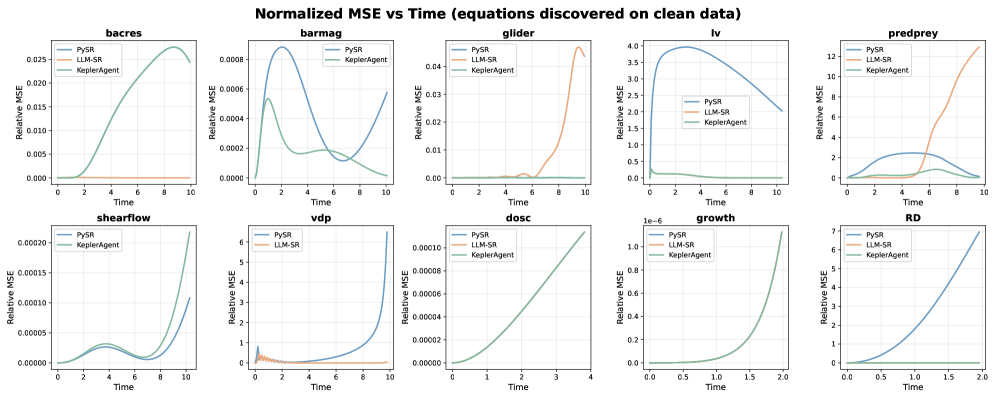
## Chart Type: Multiple Line Charts ### Overview The image contains a series of line charts comparing the performance of three different methods (PySR, LLM-SR, and KeplerAgent) in discovering equations on clean data. The charts display the Normalized Mean Squared Error (MSE) over time for various systems or models, including 'bacres', 'barmag', 'glider', 'lv', 'predprey', 'shearflow', 'vdp', 'dosc', 'growth', and 'RD'. ### Components/Axes * **Title:** Normalized MSE vs Time (equations discovered on clean data) * **X-axis:** Time (with varying scales depending on the chart, ranging from 0 to 10 in most cases, but 0 to 2 for 'growth' and 'RD', and 0 to 4 for 'dosc') * **Y-axis:** Relative MSE (with varying scales depending on the chart) * **Legend:** Located in the top-left corner of each subplot. * PySR (Blue line) * LLM-SR (Orange line) * KeplerAgent (Green line) ### Detailed Analysis **1. bacres** * X-axis: Time (0 to 10) * Y-axis: Relative MSE (0 to 0.025) * PySR: Flat line at approximately 0. * LLM-SR: Flat line at approximately 0. * KeplerAgent: Starts at 0, increases sharply to a peak around Time = 8 (Relative MSE ~ 0.026), then decreases slightly. **2. barmag** * X-axis: Time (0 to 10) * Y-axis: Relative MSE (0 to 0.0008) * PySR: Starts high (Relative MSE ~ 0.0008), decreases to a minimum around Time = 2, then increases again. * KeplerAgent: Starts low, increases to a peak around Time = 5, then decreases. **3. glider** * X-axis: Time (0 to 10) * Y-axis: Relative MSE (0 to 0.04) * PySR: Flat line at approximately 0. * LLM-SR: Starts at 0, remains low until Time = 7, then increases sharply to a peak around Time = 9 (Relative MSE ~ 0.04). * KeplerAgent: Flat line at approximately 0. **4. lv** * X-axis: Time (0 to 10) * Y-axis: Relative MSE (0 to 4.0) * PySR: Starts high (Relative MSE ~ 4.0), decreases sharply to a minimum around Time = 2, then increases slightly. * LLM-SR: Not present in the legend, but there is an orange line. * KeplerAgent: Flat line at approximately 0. **5. predprey** * X-axis: Time (0 to 10) * Y-axis: Relative MSE (0 to 12) * PySR: Starts high (Relative MSE ~ 4.0), decreases to a minimum around Time = 7, then increases slightly. * LLM-SR: Starts at 0, increases sharply after Time = 6 to a peak around Time = 10 (Relative MSE ~ 12). * KeplerAgent: Flat line at approximately 0. **6. shearflow** * X-axis: Time (0 to 10) * Y-axis: Relative MSE (0 to 0.00020) * PySR: Starts low, increases to a peak around Time = 2, decreases to a minimum around Time = 6, then increases sharply. * KeplerAgent: Starts low, increases to a peak around Time = 2, decreases to a minimum around Time = 6, then increases sharply. * LLM-SR: Not present in the legend, but there is an orange line. **7. vdp** * X-axis: Time (0 to 10) * Y-axis: Relative MSE (0 to 6) * PySR: Starts low, increases sharply. * LLM-SR: Starts high, decreases sharply, then remains relatively constant. **8. dosc** * X-axis: Time (0 to 4) * Y-axis: Relative MSE (0 to 0.00010) * PySR: Starts low, increases linearly. * LLM-SR: Starts low, increases linearly. * KeplerAgent: Starts low, increases linearly. **9. growth** * X-axis: Time (0 to 2) * Y-axis: Relative MSE (1e-6 to 1.0e-6) * PySR: Starts low, increases exponentially. * LLM-SR: Starts low, increases exponentially. * KeplerAgent: Starts low, increases exponentially. **10. RD** * X-axis: Time (0 to 2) * Y-axis: Relative MSE (0 to 7) * PySR: Starts low, increases exponentially. * LLM-SR: Flat line at approximately 0. * KeplerAgent: Flat line at approximately 0. ### Key Observations * PySR and KeplerAgent often show contrasting performance, with one having a high initial MSE that decreases over time while the other remains consistently low. * LLM-SR tends to have a delayed increase in MSE for some systems, suggesting a period of stability before diverging. * For some systems (e.g., 'growth'), all three methods exhibit similar exponential increases in MSE. * The scales of the Y-axes vary significantly across the charts, indicating different levels of difficulty in discovering equations for each system. ### Interpretation The charts provide a comparative analysis of three different methods for equation discovery on clean data. The Normalized MSE vs. Time plots illustrate how the accuracy of each method changes over time for various systems. The data suggests that the performance of each method is highly dependent on the specific system being modeled. In some cases, one method consistently outperforms the others (e.g., KeplerAgent for 'bacres'), while in other cases, the methods exhibit more complex and time-dependent behavior. The varying scales of the Y-axes highlight the different levels of difficulty associated with each system, suggesting that some systems are inherently more challenging to model accurately. The trends observed in these charts can inform the selection of appropriate equation discovery methods for different types of systems and provide insights into the strengths and weaknesses of each approach.

## Chart: Normalized MSE vs Time (equations discovered on clean data) ### Overview The image presents a 3x3 grid of line charts, each displaying the Normalized Mean Squared Error (MSE) against Time. Each chart represents a different equation/system ("barcres", "barmag", "glider", "lv", "predprey", "shearflow", "vdp", "doc", "growth", "RD"). Three different methods ("PySR", "LLM-SR", "KeplerAgent") are compared within each chart. The charts aim to visualize the performance of each method in discovering equations from clean data, with lower MSE indicating better performance. ### Components/Axes * **Title:** "Normalized MSE vs Time (equations discovered on clean data)" - positioned at the top center of the image. * **X-axis Label:** "Time" - common to all subplots, ranging from 0 to 10 (except for "growth" and "RD" which range to 1.5 and 2.0 respectively). * **Y-axis Label:** "Relative MSE" - common to all subplots, with varying scales. * **Legend:** Each subplot has a legend in the top-right corner, identifying the lines representing "PySR" (blue), "LLM-SR" (orange), and "KeplerAgent" (green). * **Subplot Titles:** Each subplot is labeled with the name of the equation/system being analyzed: "barcres", "barmag", "glider", "lv", "predprey", "shearflow", "vdp", "doc", "growth", "RD". ### Detailed Analysis or Content Details Here's a breakdown of each subplot, including approximate data points and trend descriptions: 1. **barcres:** * PySR: Line slopes downward, starting at approximately 0.025 and decreasing to approximately 0.001 at Time = 10. * LLM-SR: Line is relatively flat, around 0.00005 throughout the time range. * KeplerAgent: Line starts at approximately 0.02 and decreases to approximately 0.002 at Time = 10. 2. **barmag:** * PySR: Line is nearly flat, around 0.00002 throughout the time range. * LLM-SR: Line slopes downward, starting at approximately 0.00008 and decreasing to approximately 0.00001 at Time = 10. * KeplerAgent: Line is relatively flat, around 0.00003 throughout the time range. 3. **glider:** * PySR: Line slopes downward, starting at approximately 0.04 and decreasing to approximately 0.005 at Time = 10. * LLM-SR: Line is relatively flat, around 0.015 throughout the time range. * KeplerAgent: Line is relatively flat, around 0.02 throughout the time range. 4. **lv:** * PySR: Line slopes downward, starting at approximately 3.5 and decreasing to approximately 0.1 at Time = 10. * LLM-SR: Line is relatively flat, around 0.5 throughout the time range. * KeplerAgent: Line is relatively flat, around 1.5 throughout the time range. 5. **predprey:** * PySR: Line slopes downward, starting at approximately 12 and decreasing to approximately 0.5 at Time = 10. * LLM-SR: Line is relatively flat, around 2 throughout the time range. * KeplerAgent: Line is relatively flat, around 5 throughout the time range. 6. **shearflow:** * PySR: Line slopes downward, starting at approximately 0.002 and decreasing to approximately 0.00001 at Time = 10. * LLM-SR: Line is relatively flat, around 0.00005 throughout the time range. * KeplerAgent: Line is relatively flat, around 0.0001 throughout the time range. 7. **vdp:** * PySR: Line slopes downward, starting at approximately 0.0001 and decreasing to approximately 0.000005 at Time = 10. * LLM-SR: Line is relatively flat, around 0.00002 throughout the time range. * KeplerAgent: Line is relatively flat, around 0.00003 throughout the time range. 8. **doc:** * PySR: Line slopes downward, starting at approximately 0.00001 and decreasing to approximately 0.000001 at Time = 10. * LLM-SR: Line is relatively flat, around 0.000005 throughout the time range. * KeplerAgent: Line is relatively flat, around 0.000008 throughout the time range. 9. **growth:** * PySR: Line slopes downward, starting at approximately 1.0 and decreasing to approximately 0.05 at Time = 2.0. * LLM-SR: Line is relatively flat, around 0.2 throughout the time range. * KeplerAgent: Line is relatively flat, around 0.5 throughout the time range. 10. **RD:** * PySR: Line slopes downward, starting at approximately 0.1 and decreasing to approximately 0.01 at Time = 2.0. * LLM-SR: Line is relatively flat, around 0.03 throughout the time range. * KeplerAgent: Line is relatively flat, around 0.05 throughout the time range. ### Key Observations * PySR generally exhibits a decreasing MSE over time across all equations, suggesting it improves its equation discovery as time progresses. * LLM-SR tends to have relatively flat MSE curves, indicating consistent performance without significant improvement or degradation over time. * KeplerAgent also shows relatively flat MSE curves, but generally with higher values than LLM-SR. * The scale of the Y-axis varies significantly between subplots, indicating different levels of difficulty in discovering equations for each system. "lv" and "predprey" have the highest MSE values, suggesting these systems are the most challenging. * "barmag" and "doc" have the lowest MSE values, suggesting these systems are the easiest to discover equations for. ### Interpretation The charts demonstrate a comparison of three methods (PySR, LLM-SR, and KeplerAgent) in their ability to discover equations from clean data. PySR consistently shows improvement over time, suggesting it benefits from longer computation or more data. LLM-SR provides stable, but not necessarily optimal, performance. KeplerAgent falls between the two, offering moderate performance without significant improvement. The varying scales of the Y-axis highlight the complexity of the different equations/systems. Systems with higher initial and final MSE values (like "lv" and "predprey") are more difficult to model, while those with lower values (like "barmag" and "doc") are easier. The consistent flatness of the LLM-SR curves could indicate a limitation in its ability to refine its equation discovery process over time, or that it quickly reaches a stable solution. The decreasing trend of PySR suggests an iterative refinement process. The differences in performance across the different systems suggest that the choice of method may depend on the specific characteristics of the data and the complexity of the underlying equation.

## Chart Type: Multi-Panel Line Chart (Normalized MSE vs Time) ### Overview The image displays a 2x5 grid of line charts, each comparing the performance of three different methods (PySR, LLM-SR, KeplerAgent) over time for a specific equation discovery task. The overarching title is "Normalized MSE vs Time (equations discovered on clean data)". Each subplot represents a different target equation or system, identified by a short title. The y-axis represents "Relative MSE" (Mean Squared Error), and the x-axis represents "Time". The charts illustrate how the error of the discovered equations evolves over time for each method. ### Components/Axes * **Main Title:** "Normalized MSE vs Time (equations discovered on clean data)" * **Subplot Titles (Top Row, Left to Right):** `bacres`, `barmag`, `glider`, `lv`, `predprey` * **Subplot Titles (Bottom Row, Left to Right):** `shearflow`, `vdp`, `dosc`, `growth`, `RD` * **Axes Labels (Consistent across all subplots):** * **X-axis:** "Time" * **Y-axis:** "Relative MSE" * **Legend (Present in each subplot):** * **PySR:** Blue line * **LLM-SR:** Orange line * **KeplerAgent:** Green line * **Placement:** Typically in the top-left or top-right corner of each subplot's plotting area. * **Axis Scales:** The scales for both Time and Relative MSE vary significantly between subplots, indicating different magnitudes of error and time ranges for each equation. ### Detailed Analysis **Subplot 1: `bacres`** * **Trend:** PySR (blue) shows a steep, concave-down increase in MSE, peaking around Time=8 before slightly declining. LLM-SR (orange) and KeplerAgent (green) remain flat near zero MSE throughout. * **Key Points:** PySR MSE rises from ~0 to a peak of ~0.025. The other two methods are negligible. **Subplot 2: `barmag`** * **Trend:** PySR (blue) has a sharp, narrow peak early (Time~2), then declines and rises again later. LLM-SR (orange) has a broader, lower peak around Time~1.5. KeplerAgent (green) shows a moderate, broad peak around Time~2. * **Key Points:** PySR peak MSE ~0.0008. LLM-SR peak ~0.0005. KeplerAgent peak ~0.0005. **Subplot 3: `glider`** * **Trend:** PySR (blue) and KeplerAgent (green) are flat near zero. LLM-SR (orange) shows a dramatic, exponential-like increase starting around Time=6. * **Key Points:** LLM-SR MSE rises from ~0 to >0.04 by Time=10. **Subplot 4: `lv` (Lotka-Volterra)** * **Trend:** PySR (blue) starts high (~3.8), peaks near Time=3 (~4.0), then declines steadily. LLM-SR (orange) and KeplerAgent (green) are flat near zero. * **Key Points:** PySR MSE is orders of magnitude higher than the others. **Subplot 5: `predprey`** * **Trend:** PySR (blue) has a low, broad hump peaking around Time=4 (~2.0). LLM-SR (orange) shows a sharp, exponential increase starting around Time=6, reaching >12. KeplerAgent (green) is flat near zero. * **Key Points:** LLM-SR error becomes extremely large. PySR error is moderate. KeplerAgent performs best. **Subplot 6: `shearflow`** * **Trend:** PySR (blue) and KeplerAgent (green) follow very similar paths: a small hump around Time=4, a dip, then a sharp rise after Time=8. KeplerAgent's rise is steeper. * **Key Points:** Both end with MSE ~0.00010-0.00020. The y-axis scale is very small (1e-4). **Subplot 7: `vdp` (Van der Pol oscillator)** * **Trend:** PySR (blue) is flat near zero. LLM-SR (orange) shows a sharp, exponential increase starting around Time=8. * **Key Points:** LLM-SR MSE rises from ~0 to >6 by Time=10. **Subplot 8: `dosc`** * **Trend:** PySR (blue) and KeplerAgent (green) are flat near zero. LLM-SR (orange) shows a smooth, accelerating increase. * **Key Points:** LLM-SR MSE rises from 0 to ~0.00010 by Time=4. The y-axis scale is very small (1e-4). **Subplot 9: `growth`** * **Trend:** PySR (blue) and KeplerAgent (green) are flat near zero. LLM-SR (orange) shows a very sharp, exponential increase. * **Key Points:** LLM-SR MSE rises from 0 to >1.0 by Time=2.0. The y-axis has a multiplier of 1e-6, so values are on the order of 1e-6. **Subplot 10: `RD` (Reaction-Diffusion?)** * **Trend:** PySR (blue) shows a smooth, accelerating increase. LLM-SR (orange) and KeplerAgent (green) are flat near zero. * **Key Points:** PySR MSE rises from 0 to >7 by Time=2.0. ### Key Observations 1. **Method Performance is Highly Equation-Dependent:** No single method (PySR, LLM-SR, KeplerAgent) is universally superior. Their relative performance flips dramatically between different equations. 2. **Catastrophic Failure Modes:** LLM-SR exhibits extreme, exponential error growth in several cases (`glider`, `predprey`, `vdp`, `growth`), suggesting instability or poor generalization for those dynamics. 3. **Stability of KeplerAgent:** KeplerAgent (green) often remains stable with low error (flat line near zero), particularly in `bacres`, `lv`, `predprey`, `dosc`, `growth`, and `RD`. It is rarely the worst performer. 4. **PySR's Variable Performance:** PySR (blue) shows the widest range of behaviors: it can be the worst (`lv`, `RD`), have moderate error (`predprey`), or perform well (`bacres`, `glider`). 5. **Scale Discrepancies:** The y-axis scales differ by orders of magnitude (e.g., `shearflow` max ~2e-4 vs. `predprey` max >12), indicating the inherent difficulty or error magnitude varies greatly across the tested equations. ### Interpretation This collection of charts serves as a benchmark comparison of symbolic regression or equation discovery algorithms. The data suggests that the choice of algorithm must be carefully matched to the problem domain. * **Underlying Pattern:** The plots reveal a trade-off between methods that may have higher initial error but remain stable (KeplerAgent) versus methods that can achieve very low error but risk catastrophic divergence for certain equation types (LLM-SR, and to a lesser extent, PySR). * **Equation Complexity:** The equations where LLM-SR fails spectacularly (`glider`, `predprey`, `vdp`) likely represent more complex, nonlinear dynamical systems. Its success on simpler or different types of equations (`shearflow`, `dosc`) indicates its performance is not uniformly poor. * **Investigative Insight:** A researcher viewing this would conclude that robustness (KeplerAgent) and peak accuracy (variable across methods) are separate axes of performance. The ideal algorithm would combine the stability of KeplerAgent with the peak accuracy potential shown by the best-performing method in each individual plot. The charts highlight specific failure cases (`predprey` for LLM-SR, `lv` for PySR) that warrant deeper investigation into why those methods struggle with those particular mathematical structures.

## Line Graphs: Normalized MSE vs Time (Equations Discovered on Clean Data) ### Overview The image contains 10 line graphs comparing the performance of three methods—PySR (blue), LLM-SR (orange), and KeplerAgent (green)—across different dynamical systems. Each graph plots **Relative Mean Squared Error (MSE)** against **Time** (0–10, except for "growth" and "RD" which end at 2). The y-axis scales vary per dataset, with values ranging from 1e-6 to 12. Trends indicate how each method's error evolves over time. --- ### Components/Axes - **X-axis**: Time (0–10 for most datasets; 0–2 for "growth" and "RD"). - **Y-axis**: Relative MSE (dataset-specific scales, e.g., 0–0.025 for "bacres", 0–12 for "predprey"). - **Legend**: - Blue = PySR - Orange = LLM-SR - Green = KeplerAgent - **Datasets** (graph titles): bacres, barmag, glider, lv, predprey, shearflow, vdp, dosc, growth, RD. --- ### Detailed Analysis #### bacres - **PySR**: Flat line at ~0.0002. - **LLM-SR**: Flat line at ~0.0001. - **KeplerAgent**: Starts near 0, rises sharply to ~0.025 at t=8, then drops to ~0.015 at t=10. #### barmag - **PySR**: Peaks at ~0.0008 at t=2, drops to ~0.0002 by t=10. - **KeplerAgent**: Peaks at ~0.0006 at t=2, then declines to ~0.0001 by t=10. #### glider - **PySR**: Flat line at ~0.0001. - **LLM-SR**: Flat until t=8, then spikes to ~0.04 at t=10. - **KeplerAgent**: Flat line at ~0.0001. #### lv - **PySR**: Peaks at ~3.5 at t=2, declines to ~2.0 by t=10. - **LLM-SR**: Flat line at ~0.0. - **KeplerAgent**: Flat line at ~0.0. #### predprey - **PySR**: Peaks at ~2.0 at t=4, drops to ~0.5 at t=10. - **LLM-SR**: Flat until t=6, then rises sharply to ~12 at t=10. - **KeplerAgent**: Peaks at ~1.0 at t=6, then drops to ~0.2 at t=10. #### shearflow - **PySR**: Peaks at ~0.00015 at t=4, drops to ~0.0001 by t=10. - **KeplerAgent**: Peaks at ~0.00015 at t=4, then rises to ~0.0002 at t=10. #### vdp - **PySR**: Peaks at ~6 at t=2, drops to ~1 at t=10. - **LLM-SR**: Flat line at ~0.0. - **KeplerAgent**: Flat line at ~0.0. #### dosc - **PySR**: Flat line at ~0.0. - **LLM-SR**: Flat line at ~0.0. - **KeplerAgent**: Linear rise from ~0.0 to ~0.0001 at t=4. #### growth - **PySR**: Flat line at ~0.0. - **LLM-SR**: Flat line at ~0.0. - **KeplerAgent**: Linear rise from ~0.0 to ~1.0 at t=2. #### RD - **PySR**: Linear rise from ~0.0 to ~7 at t=2. - **LLM-SR**: Flat line at ~0.0. - **KeplerAgent**: Flat line at ~0.0. --- ### Key Observations 1. **KeplerAgent** generally maintains low MSE in most datasets (e.g., "barmag", "glider", "shearflow") but struggles in "bacres" and "predprey". 2. **PySR** performs well in "lv" and "vdp" but shows instability in "predprey" and "RD". 3. **LLM-SR** fails catastrophically in "predprey" (spikes to 12) and "glider" (spikes to 0.04). 4. **Time horizons** vary: "growth" and "RD" end at t=2, while others extend to t=10. --- ### Interpretation - **KeplerAgent** demonstrates robustness in simple systems (e.g., "barmag", "shearflow") but falters in complex or chaotic systems like "predprey" and "lv". - **PySR** excels in systems with smooth dynamics ("lv", "vdp") but struggles with oscillatory or high-dimensional systems ("predprey", "RD"). - **LLM-SR** is unreliable in "predprey" and "glider", suggesting poor generalization to certain dynamical regimes. - The divergence in performance highlights the importance of method selection based on system complexity and noise characteristics. All trends align with the legend colors, confirming accurate data attribution. No textual elements or non-English content are present.