## Histogram: Distribution Plot ### Overview The image is a histogram overlaid with a probability density function (PDF). The histogram consists of vertical bars representing the frequency distribution of data, while the PDF is a smooth curve that approximates the distribution. The data appears to be centered around zero. ### Components/Axes * **X-axis:** Ranges from -0.4 to 0.8, with tick marks at -0.4, -0.2, 0, 0.2, 0.4, 0.6, and 0.8. The x-axis likely represents the values of the variable being measured. * **Y-axis:** Ranges from 0 to 0.005, with tick marks at 0, 0.001, 0.002, 0.003, 0.004, and 0.005. The y-axis represents the frequency or density of the data. * **Histogram:** A series of vertical bars, with the highest concentration of bars around 0. * **PDF Curve:** A smooth, bell-shaped curve overlaid on the histogram, centered around 0. ### Detailed Analysis * **Histogram Bars:** The bars are concentrated around 0, indicating that most of the data points are close to 0. The height of the bars varies, with the tallest bar reaching approximately 0.005. * **PDF Curve:** The curve closely follows the shape of the histogram, indicating a good fit. The peak of the curve is at 0, and it gradually decreases as it moves away from 0 in both directions. ### Key Observations * The data is heavily concentrated around 0. * The distribution appears to be approximately normal, as suggested by the bell-shaped PDF curve. * There are some data points that are further away from 0, but they are relatively infrequent. ### Interpretation The histogram and PDF suggest that the data is centered around zero and follows a roughly normal distribution. This could represent a variety of phenomena, such as measurement errors, fluctuations around a target value, or the distribution of residuals in a statistical model. The concentration of data around zero suggests that the underlying process is stable and well-controlled. The presence of some data points further away from zero indicates that there are occasional deviations from the norm, but they are relatively rare.

\n ## Chart: Histogram with Density Curve ### Overview The image displays a histogram with an overlaid density curve. The histogram represents the distribution of a single variable, with values ranging approximately from -0.4 to 0.8. The density curve provides a smoothed estimate of the underlying probability distribution. ### Components/Axes * **X-axis:** Ranges from -0.4 to 0.8, with tick marks at intervals of 0.2. The axis is labeled, but the label is not visible in the image. * **Y-axis:** Ranges from 0 to 0.005, with tick marks at intervals of 0.001. The axis is labeled, but the label is not visible in the image. The Y-axis represents frequency or density. * **Histogram:** Composed of numerous vertical bars representing the frequency of values within specific bins. * **Density Curve:** A smooth, black curve overlaid on the histogram, estimating the probability density function of the data. ### Detailed Analysis The histogram shows a highly skewed distribution. The majority of the data is concentrated around 0, with a sharp peak. There is a long tail extending towards the right (positive values). * **Peak:** The highest frequency occurs around x = 0, with a density of approximately 0.0045. * **Left Side:** From -0.4 to approximately -0.1, the density is very low, close to 0. * **Right Side:** From approximately 0.1 to 0.8, the density decreases gradually, with some minor fluctuations. * **Density Curve Trend:** The density curve closely follows the shape of the histogram, peaking at x = 0 and decreasing as it moves away from 0. The curve is smooth and provides a general representation of the distribution. ### Key Observations * The distribution is strongly right-skewed. * There is a high concentration of data points near 0. * The density decreases rapidly as the values move away from 0 in both directions, but more slowly towards positive values. * The histogram has a large number of narrow bins, providing a detailed view of the distribution. ### Interpretation The data suggests a variable where values are predominantly close to zero, with a smaller number of significantly positive values. This could represent a variety of phenomena, such as: * **Residuals from a regression model:** If this is a histogram of residuals, it suggests the model may not be perfectly capturing the relationship between variables, as the residuals are not normally distributed. * **Changes or differences:** The variable could represent changes or differences between two measurements, where most changes are small and close to zero, but some are larger and positive. * **Rates or proportions:** The variable could represent a rate or proportion, where most values are small, but some are larger. The density curve provides a smoothed representation of the distribution, highlighting the overall shape and central tendency. The skewness indicates that the mean and median of the distribution are likely to be different, with the mean being greater than the median. The presence of a long tail suggests that there may be outliers or extreme values in the data. Without knowing the context of the variable, it is difficult to draw more specific conclusions.

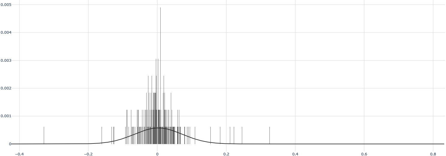
## Histogram with Overlaid Probability Density Curve ### Overview The image displays a statistical chart consisting of a histogram (vertical bars) overlaid with a smooth probability density function (PDF) curve. The chart visualizes the distribution of a dataset. There are no explicit titles, axis labels, or legends present in the image. ### Components/Axes * **X-Axis (Horizontal):** A numerical scale ranging from approximately -0.4 to 0.8. Major tick marks are visible at intervals of 0.2 (e.g., -0.4, -0.2, 0, 0.2, 0.4, 0.6, 0.8). The axis line itself is solid black. * **Y-Axis (Vertical):** A numerical scale representing frequency density, ranging from 0 to 0.005. Major tick marks are present at intervals of 0.001 (e.g., 0, 0.001, 0.002, 0.003, 0.004, 0.005). * **Histogram Bars:** Numerous thin, vertical gray bars. Their height corresponds to the frequency density of data points within specific bins along the x-axis. * **Probability Density Curve:** A single, smooth, solid black line overlaid on the histogram. It represents a theoretical or fitted distribution model for the data. * **Grid:** A faint, light-gray grid is present in the background, with lines corresponding to the major ticks on both axes. ### Detailed Analysis * **Data Distribution (Histogram):** * The histogram bars are densely clustered around the x-axis value of 0. * The highest bar (peak frequency density) is located at or very near x=0, reaching a y-value of approximately 0.0049. * The distribution appears roughly symmetric around 0. * The spread (width) of the histogram is relatively narrow. The vast majority of bars are contained between x = -0.1 and x = 0.1. * There are a few sparse, very short bars extending further out, with the leftmost visible bar near x = -0.35 and the rightmost near x = 0.35. These represent potential outliers or the tails of the distribution. * **Probability Density Curve:** * The curve is unimodal (single-peaked) and bell-shaped, characteristic of a normal (Gaussian) or similar symmetric distribution. * The peak of the curve aligns closely with x=0, matching the histogram's mode. * The peak height of the curve is approximately 0.0006 on the y-axis, which is significantly lower than the peak of the histogram bars. This suggests the curve may represent a smoothed estimate or a different normalization. * The curve tapers off smoothly towards zero on both sides, becoming negligible beyond approximately x = -0.2 and x = 0.2. ### Key Observations 1. **Central Tendency:** The data is strongly centered around zero. 2. **Low Variance/High Precision:** The data has a very narrow spread, indicating low variance or high precision in the measured variable. 3. **Symmetry:** The distribution is visually symmetric. 4. **Outliers:** A few data points exist in the tails (e.g., near -0.35 and +0.35), but they are extremely rare compared to the central cluster. 5. **Model Fit:** The overlaid smooth curve captures the general symmetric, bell-shaped nature of the data but does not match the extreme peakedness (kurtosis) of the histogram. The histogram is more "spiky" or leptokurtic than the fitted curve. ### Interpretation This chart demonstrates a dataset where the measured values are highly concentrated around a mean of zero, with very small deviations. This pattern is typical of: * **Residuals from a well-fitting statistical model,** where most errors are near zero. * **Measurement noise** from a high-precision instrument. * **Returns of a very stable financial asset** over a short period. * **Differences between matched pairs** in a controlled experiment showing minimal effect. The discrepancy between the sharp histogram peak and the smoother, lower curve suggests the underlying data distribution may have heavier tails or a sharper peak than the theoretical model (e.g., a normal distribution) used to generate the curve. The presence of sparse bars in the tails (-0.35 to 0.35) confirms that while extreme values are possible, they are highly improbable compared to values near zero. The lack of axis labels prevents definitive identification of the variable being measured, but the statistical behavior is clearly one of high central tendency and low dispersion.

## Line Graph: Normal Distribution with Error Bars ### Overview The image depicts a line graph representing a normal distribution curve with superimposed error bars. The x-axis spans from -0.4 to 0.8, while the y-axis ranges from 0 to 0.005. The graph includes a smooth black line forming a bell-shaped curve and vertical error bars clustered around the center. The legend is positioned at the bottom-right but contains no visible text or labels. ### Components/Axes - **X-Axis**: Labeled with approximate values at intervals: -0.4, -0.2, 0, 0.2, 0.4, 0.6, 0.8. No explicit title is visible. - **Y-Axis**: Labeled with approximate values at intervals: 0.001, 0.002, 0.003, 0.004, 0.005. No explicit title is visible. - **Legend**: Located at the bottom-right corner but empty (no labels or color keys). - **Grid**: Light gray grid lines span the entire plot area. - **Main Line**: A smooth black curve forming a normal distribution, peaking at x=0 with a y-value of approximately 0.002. - **Error Bars**: Vertical black lines clustered around the center (x=0), with heights decreasing symmetrically toward the edges. Heights range from ~0.001 to ~0.004. ### Detailed Analysis - **Main Line**: The curve follows a Gaussian distribution, peaking at x=0 (y≈0.002) and tapering off to near-zero values at x=±0.4. The curve is symmetric, with no visible anomalies. - **Error Bars**: - Tallest bars (~0.004) are centered at x=0, decreasing in height as x moves away from 0. - Bars become sparser and shorter beyond x=±0.2, with minimal presence beyond x=±0.4. - Heights suggest variability in measurements, with standard deviations likely decreasing away from the mean. ### Key Observations 1. **Symmetry**: The distribution and error bars are symmetric about x=0. 2. **Peak Variability**: The highest error bars (0.004) align with the curve’s maximum, indicating maximum uncertainty at the mean. 3. **Tapered Distribution**: Both the curve and error bars diminish rapidly beyond x=±0.2, suggesting limited data or confidence in extreme values. 4. **Missing Legend Text**: The legend’s absence of labels implies either a generic plot or omitted contextual information. ### Interpretation The graph likely represents a dataset with a central tendency around x=0, where measurements cluster most densely. The error bars’ heights and distribution suggest: - **Highest Uncertainty at the Mean**: The tallest error bars at x=0 imply greater variability or measurement error near the central value. - **Confidence in Central Values**: The curve’s peak and dense error bars indicate strong agreement in measurements around x=0. - **Rapid Decline in Confidence**: The sharp drop in error bar heights and curve amplitude beyond x=±0.2 suggests limited data or lower confidence in extreme values. The absence of a legend title or axis labels reduces interpretability, but the visual structure strongly aligns with a normal distribution model. The error bars may represent standard deviations or confidence intervals, though their exact meaning remains unclear without textual clarification.