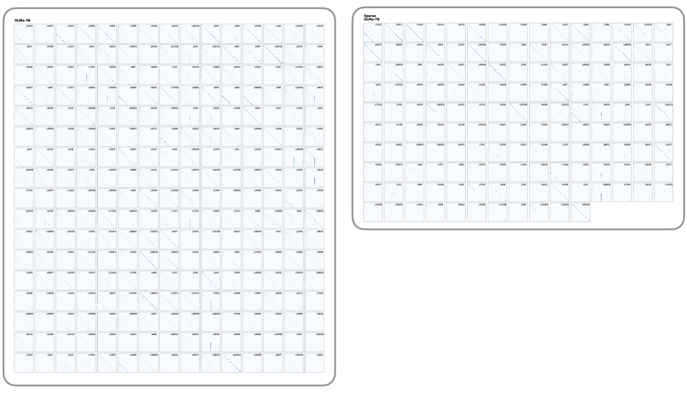
## Diagram: Attention Head Visualizations - OLMo-7B vs. Sparse OLMo-7B
### Overview
This image presents a side-by-side technical visualization of attention matrices (or weight patterns) for two variations of a Large Language Model: a standard "OLMo-7B" and a "Sparse OLMo-7B". The image is divided into two distinct panels, each containing a grid of smaller square plots. Each small plot represents the attention pattern of a specific "Head" within a specific "Layer" of the transformer architecture. The visualizations demonstrate the effect of sparsification (pruning) on the model's attention mechanisms.
### Components/Axes
* **Left Panel (Dense Model):**
* **Title:** "OLMo-7B" (located top-left of the panel).
* **Structure:** A perfect 16 $\times$ 16 grid of square plots. Totaling 256 plots.
* **Right Panel (Sparse Model):**
* **Title:** "Sparse OLMo-7B" (located top-left of the panel).
* **Structure:** An incomplete grid consisting of 10 rows and 16 columns. The first 9 rows are full (16 plots each), and the 10th row contains 11 plots. Totaling 155 plots.
* **Individual Plots (Sub-components):**
* **Axes (Implicit):** In standard attention maps, the X-axis represents the "Key" token sequence position, and the Y-axis represents the "Query" token sequence position. The origin (0,0) is at the top-left of each square.
* **Data Points:** Dark blue/black pixels against a white/light-blue background indicate high attention weights or activation values between specific token positions.
* **Labels:** Every single plot has a microscopic alphanumeric label in its top-right corner following the format `L[#]H[#]`, where `L` stands for Layer and `H` stands for Head.
### Content Details & Trend Verification
#### 1. Left Panel: OLMo-7B (Systematic Sample)
* **Labeling Pattern:** Due to image resolution, not every label is perfectly legible, but a clear structural pattern emerges upon close inspection of the grid edges:
* **Columns (Left to Right):** Represent Heads 0 through 15 (`H0` to `H15`).
* **Rows (Top to Bottom):** Represent *even-numbered* Layers. Row 1 is `L0`, Row 2 is `L2`, Row 3 is `L4`, down to Row 16 which is `L30`.
* *Transcription Example (Top Row):* `L0H0`, `L0H1`, `L0H2` ... `L0H15`.
* *Transcription Example (First Column):* `L0H0`, `L2H0`, `L4H0` ... `L30H0`.
* **Visual Trends:**
* **Diagonal Lines:** The vast majority of the plots feature a distinct, sharp line running diagonally from the top-left to the bottom-right. This indicates causal or local attention, where a token primarily attends to itself or immediately preceding tokens.
* **Vertical Lines:** Several plots (e.g., in the 4th, 8th, and 14th columns across various layers) show distinct vertical lines, usually on the far left side of the plot. This indicates "sink" attention, where all tokens in the sequence attend heavily to the first few tokens (often a Beginning-of-Sequence token).
* **Sparsity within Dense:** Even in this standard model, some heads (e.g., `L10H3`, `L20H12`) appear mostly blank, indicating they contribute very little distinct routing information.
#### 2. Right Panel: Sparse OLMo-7B (Retained Subset)
* **Labeling Pattern:** Unlike the left panel, the right panel does *not* follow a uniform grid of sequential layers and heads. The labels represent the specific subset of heads that survived the sparsification process.
* The total number of plots is exactly 155.
* The labels appear to be sorted sequentially by Layer and then Head, but with massive gaps.
* *Transcription Example (Row 1):* The first row appears to retain many of the early layer heads, starting with `L0H0`, `L0H1`, etc.
* *Transcription Example (Scattered):* Moving down the rows, the layer numbers jump irregularly, indicating that the pruning algorithm selectively dropped specific heads across the entire network based on a specific criteria (likely importance or magnitude), rather than dropping entire layers uniformly.
* **Visual Trends:**
* The fundamental visual patterns (diagonals and verticals) remain identical to the left panel.
* The heads retained in this sparse model predominantly feature very sharp, highly defined diagonal lines. Heads that were "blank" or diffuse in the standard model appear to have been purged.
### Key Observations
1. **Volume Reduction:** The most striking observation is the difference in volume. The left panel shows a 256-head sample of the dense model (which likely has 1024 total heads if it's a 32-layer, 32-head architecture). The right panel shows only 155 heads *in total* for the sparse model. This implies a massive pruning ratio (potentially removing over 80% of the attention heads).
2. **Pattern Preservation:** Despite the massive reduction in the number of heads, the fundamental geometric patterns of attention (causal diagonals and BOS-token verticals) are strictly preserved in the remaining heads.
### Interpretation
This image serves as visual proof of a model pruning or sparsification experiment.
In Large Language Models, it is a known phenomenon that many attention heads learn redundant features or contribute very little to the final output (often referred to as the "lottery ticket hypothesis" or head redundancy). The left panel shows the baseline state: a vast array of heads, some with strong patterns, some weak.
The right panel ("Sparse OLMo-7B") demonstrates the result of an algorithm designed to identify and remove the "useless" heads to save compute and memory. By looking at the irregular labels and the total count (155), we can deduce that this was an *unstructured* or *semi-structured* head pruning approach. The algorithm evaluated every head individually and kept only the most critical ones.
The fact that the surviving heads in the Sparse model almost universally display strong, crisp diagonal or vertical patterns suggests that the pruning algorithm successfully identified heads with high-confidence, structured routing behaviors as the most "important" to retain, discarding heads with diffuse or noisy attention matrices.