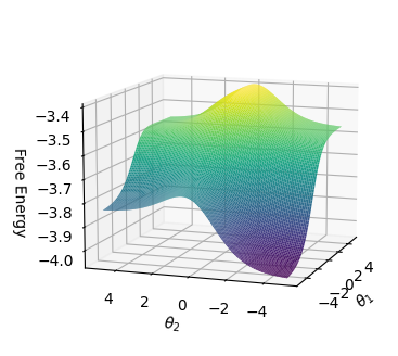
\n ## 3D Surface Plot: Free Energy Landscape ### Overview The image depicts a 3D surface plot representing a free energy landscape. The plot visualizes the relationship between two angular parameters, θ₁ and θ₂, and the corresponding free energy. The surface exhibits a complex shape with a prominent minimum and a broad maximum. ### Components/Axes * **X-axis:** θ₂ (Theta 2), ranging approximately from -4 to 4. * **Y-axis:** θ₁ (Theta 1), ranging approximately from -4 to 4. * **Z-axis:** Free Energy, ranging approximately from -3.4 to -4.0. * **Surface:** The colored surface represents the free energy value for each combination of θ₁ and θ₂. The color gradient indicates the free energy level, with yellow representing higher free energy and purple representing lower free energy. ### Detailed Analysis The surface shows a clear minimum around θ₁ ≈ 0 and θ₂ ≈ 0. The free energy at this minimum is approximately -3.9. The surface rises to a broad maximum along the θ₂ axis, peaking around θ₂ ≈ 4 and θ₁ ≈ 0. The free energy at this maximum is approximately -3.4. The surface slopes downwards as θ₁ moves away from 0 in both positive and negative directions. The surface is relatively smooth, with no sharp discontinuities or abrupt changes. ### Key Observations * **Minimum:** A distinct minimum in free energy exists near θ₁ = 0 and θ₂ = 0, suggesting a stable state or configuration. * **Maximum:** A broad maximum exists along the θ₂ axis, indicating a less stable region. * **Gradient:** The color gradient clearly shows the variation in free energy across the landscape. * **Symmetry:** The plot appears roughly symmetric about the θ₁ = 0 axis. ### Interpretation This plot likely represents the free energy landscape of a system with two rotational degrees of freedom, θ₁ and θ₂. The minimum in free energy corresponds to the most stable configuration of the system, while the maximum represents a less stable configuration. The shape of the landscape dictates the system's dynamics; the system will tend to move towards the minimum, but may encounter barriers along the way. The symmetry suggests that the system's behavior is not significantly affected by the sign of θ₁. This type of plot is commonly used in fields like molecular dynamics, statistical mechanics, and machine learning to visualize and understand the energy landscape of complex systems. The plot suggests that the system is most stable when both angles are close to zero, and that deviations from this configuration increase the free energy. The broad maximum indicates a region where the system is less likely to reside, but can still access.