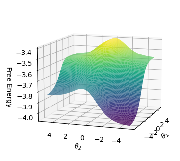
## 3D Surface Plot: Free Energy Landscape over Parameters θ₁ and θ₂ ### Overview The image displays a three-dimensional surface plot visualizing a scalar field, "Free Energy," as a function of two independent parameters, θ₁ and θ₂. The plot uses a color gradient to represent the magnitude of the Free Energy, creating a topographical map of an energy landscape. ### Components/Axes * **Vertical Axis (Z-axis):** * **Label:** "Free Energy" * **Scale:** Linear, ranging from -4.0 at the bottom to -3.4 at the top. Major tick marks are at intervals of 0.1 (-4.0, -3.9, -3.8, -3.7, -3.6, -3.5, -3.4). * **Horizontal Axis 1 (X-axis, front-left):** * **Label:** "θ₂" * **Scale:** Linear, ranging from -4 to 4. Major tick marks are at -4, -2, 0, 2, 4. * **Horizontal Axis 2 (Y-axis, front-right):** * **Label:** "θ₁" * **Scale:** Linear, ranging from -4 to 4. Major tick marks are at -4, -2, 0, 2, 4. * **Legend / Color Bar:** * **Position:** Located on the right side of the plot. * **Title:** "Free Energy" * **Scale:** A vertical gradient bar mapping color to numerical Free Energy values. The scale matches the Z-axis, from -4.0 (dark blue/purple) at the bottom to -3.4 (bright yellow) at the top. ### Detailed Analysis The surface represents a continuous function Free Energy = f(θ₁, θ₂). Its shape is characterized by: * **Global Minimum:** The lowest point on the surface (deepest blue/purple) is located approximately at coordinates **(θ₁ ≈ -2, θ₂ ≈ 2)**, where the Free Energy is near **-4.0**. * **Global Maximum:** The highest point (brightest yellow) is located approximately at the opposite corner, **(θ₁ ≈ 4, θ₂ ≈ -4)**, where the Free Energy is near **-3.4**. * **Surface Topography:** The surface forms a saddle-like shape or a valley. From the minimum at (θ₁≈-2, θ₂≈2), the energy increases as one moves away in most directions. There is a noticeable ridge or saddle point running roughly diagonally across the parameter space. * **Color Gradient:** The color transitions smoothly from dark blue/purple (lowest energy) through teal and green to yellow (highest energy), providing a direct visual correlation between position on the surface and the Free Energy value. ### Key Observations 1. **Clear Minimum:** There is a well-defined, broad minimum region in the parameter space, suggesting a stable or optimal configuration around θ₁ ≈ -2, θ₂ ≈ 2. 2. **Asymmetric Landscape:** The energy landscape is not symmetric. The gradient (rate of change) appears steeper when moving from the minimum towards the high-energy corner (θ₁=4, θ₂=-4) compared to other directions. 3. **Parameter Correlation:** The shape indicates a strong correlation between θ₁ and θ₂ in determining the Free Energy. The path of lowest energy does not follow a simple axis-aligned direction. 4. **Bounded Domain:** The plot is rendered over a square domain where both θ₁ and θ₂ range from -4 to 4. ### Interpretation This plot visualizes the "energy landscape" of a system governed by two parameters, θ₁ and θ₂. In fields like statistical mechanics, machine learning (e.g., loss landscapes), or optimization, such a plot is fundamental. * **What it demonstrates:** The system has a preferred state (the energy minimum) at specific parameter values. The surrounding landscape shows how the system's energy (or cost, or instability) changes as parameters are varied. The saddle shape is characteristic of many complex systems, indicating that there are directions in parameter space where the system is stable (moving along the valley) and directions where it is unstable (moving up the steep slopes). * **Relationship between elements:** The two parameters θ₁ and θ₂ are coupled; their joint values determine the system's state. The Free Energy is the dependent variable, a single metric summarizing the system's "goodness" or stability for a given (θ₁, θ₂) pair. * **Notable implications:** The existence of a single, broad minimum suggests the system has a robust optimal operating point. The steep rise to the maximum at (4, -4) indicates that this region of parameter space is highly unfavorable. An optimization algorithm starting from a random point would be expected to "roll down" the surface towards the dark blue minimum region. The plot provides a complete visual summary of the system's stability and the sensitivity of its state to parameter changes.