# Technical Document Extraction: Histogram Analysis
## Overview
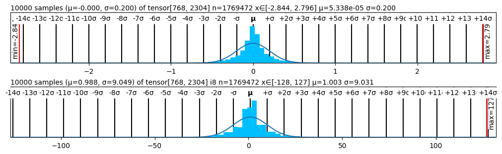
The image contains two overlaid histograms with normal distribution curves, representing statistical distributions of tensor data. Both histograms include axis labels, legends, and annotations for statistical parameters.
---
## Top Histogram
### Title
- **Text**: `10000 samples (μ=-0.000, σ=0.200) of tensor[768, 2304] n=1769472 x∈[-2.844, 2.796] μ=5.338e-05 σ=0.200`
- **Interpretation**:
- 10,000 samples drawn from a tensor with dimensions `[768, 2304]`.
- Population mean (μ) = -0.000, standard deviation (σ) = 0.200.
- Observed range: `x ∈ [-2.844, 2.796]`.
- Adjusted μ = 5.338e-05, σ = 0.200 (likely due to sampling bias or normalization).
### Axes
- **X-axis**:
- Label: Implicit (frequency bins).
- Range: `-2` to `2`.
- Markers: `-14σ` to `+14σ` in increments of `1σ` (e.g., `-14σ, -13σ, ..., +14σ`).
- **Y-axis**:
- Label: `Frequency`.
- Scale: Implicit (counts per bin).
### Legend
- **Normal Distribution Curve**:
- Dashed line with legend entry: `μ=5.338e-05 σ=0.200`.
- Color: Gray (dashed).
### Annotations
- **Min/Max**:
- Red vertical lines at `x = -2.84` (min) and `x = 2.79` (max).
- Labels: `min=-2.84`, `max=2.79`.
### Trends
- **Distribution Shape**:
- Bell-shaped histogram centered near `μ ≈ 0`.
- Overlaid normal curve matches the histogram's symmetry.
- **Spread**:
- Narrow distribution (σ = 0.200), with most data within `[-2.84, 2.79]`.
---
## Bottom Histogram
### Title
- **Text**: `10000 samples (μ=0.988, σ=9.049) of tensor[768, 2304] i8 n=1769472 x∈[-128, 127] μ=1.003 σ=9.031`
- **Interpretation**:
- 10,000 samples from a tensor with dimensions `[768, 2304]`.
- Population mean (μ) = 0.988, σ = 9.049.
- Observed range: `x ∈ [-128, 127]`.
- Adjusted μ = 1.003, σ = 9.031 (likely due to sampling bias or normalization).
### Axes
- **X-axis**:
- Label: Implicit (frequency bins).
- Range: `-100` to `100`.
- Markers: `-14σ` to `+14σ` in increments of `10σ` (e.g., `-14σ, -13σ, ..., +14σ`).
- **Y-axis**:
- Label: `Frequency`.
- Scale: Implicit (counts per bin).
### Legend
- **Normal Distribution Curve**:
- Dashed line with legend entry: `μ=1.003 σ=9.031`.
- Color: Gray (dashed).
### Annotations
- **Min/Max**:
- Red vertical lines at `x = -128` (min) and `x = 127` (max).
- Labels: `min=-128`, `max=127`.
### Trends
- **Distribution Shape**:
- Bell-shaped histogram centered near `μ ≈ 1`.
- Overlaid normal curve matches the histogram's symmetry.
- **Spread**:
- Wide distribution (σ = 9.049), with most data within `[-128, 127]`.
---
## Comparative Analysis
| Parameter | Top Histogram | Bottom Histogram |
|---------------------|---------------------|---------------------|
| **μ (Population)** | -0.000 | 0.988 |
| **σ (Population)** | 0.200 | 9.049 |
| **Adjusted μ** | 5.338e-05 | 1.003 |
| **Adjusted σ** | 0.200 | 9.031 |
| **Observed Range** | [-2.844, 2.796] | [-128, 127] |
| **σ Increment** | 1σ | 10σ |
---
## Key Observations
1. **Normalization/Adjustment**:
- Both histograms show slight adjustments to μ and σ in their legends compared to the population parameters, suggesting sampling or preprocessing effects.
2. **Scale Differences**:
- The bottom histogram spans a much larger range (`[-128, 127]`) with a higher σ, indicating greater variability in the data.
3. **Binning Strategy**:
- Top histogram uses finer bins (`1σ` increments), while the bottom uses coarser bins (`10σ` increments), affecting visual granularity.
---
## Conclusion
The histograms illustrate two distinct tensor distributions with differing central tendencies and variability. The top histogram represents a tightly clustered distribution near zero, while the bottom histogram shows a broader distribution centered slightly above zero. Both include overlaid normal curves for theoretical comparison.