## Line Chart: Test Loss vs. Compute (PF-days)
### Overview
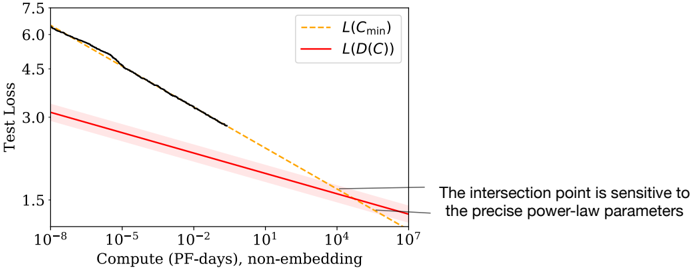
The image is a technical line chart plotting "Test Loss" against "Compute (PF-days), non-embedding" on a logarithmic x-axis. It compares two different loss functions or models, showing how their performance (loss) scales with increasing computational resources. A key annotation highlights the sensitivity of the intersection point between the two curves.
### Components/Axes
* **Chart Type:** Log-log line chart (x-axis is logarithmic, y-axis appears linear).
* **X-Axis:**
* **Label:** `Compute (PF-days), non-embedding`
* **Scale:** Logarithmic, ranging from `10^-8` to `10^7`.
* **Major Ticks:** `10^-8`, `10^-5`, `10^-2`, `10^1`, `10^4`, `10^7`.
* **Y-Axis:**
* **Label:** `Test Loss`
* **Scale:** Linear.
* **Range:** Approximately 1.5 to 7.5.
* **Major Ticks:** `1.5`, `3.0`, `4.5`, `6.0`, `7.5`.
* **Legend:** Located in the top-right quadrant of the chart area.
* `--- L(C_min)`: Represented by a dashed orange line.
* `— L(D(C))`: Represented by a solid red line with a semi-transparent red shaded area (likely indicating confidence interval or variance).
* **Unlabeled Element:** A solid black line segment is present in the upper-left portion of the chart.
* **Annotation:** A text box with an arrow pointing to the intersection of the red and dashed orange lines. The text reads: `The intersection point is sensitive to the precise power-law parameters`.
### Detailed Analysis
1. **Data Series & Trends:**
* **Black Line (Unlabeled):** Starts at the top-left of the chart (approx. Compute = `10^-8`, Loss ≈ `6.3`). It follows a steep, linear downward slope on the log-log plot, ending near (Compute ≈ `10^0`, Loss ≈ `3.0`). This indicates a strong power-law relationship where loss decreases rapidly with initial increases in compute.
* **Red Line - `L(D(C))`:** Starts lower than the black line (approx. Compute = `10^-8`, Loss ≈ `3.2`). It follows a shallower, linear downward slope. The line is accompanied by a shaded red region, suggesting a range of uncertainty. It continues across the entire x-axis range, ending near (Compute = `10^7`, Loss ≈ `1.8`).
* **Dashed Orange Line - `L(C_min)`:** Appears to be a continuation or projection. It starts where the black line ends (approx. Compute = `10^0`, Loss ≈ `3.0`) and follows a slope similar to the red line. It intersects the red line at a point indicated by the annotation.
2. **Intersection Point:** The dashed orange line `L(C_min)` and the solid red line `L(D(C))` intersect at approximately:
* **Compute:** `10^4` PF-days (10,000 PF-days).
* **Test Loss:** Approximately `2.1`.
* The annotation explicitly states this point's location is highly dependent on the underlying power-law model parameters.
### Key Observations
* **Scaling Laws:** Both primary curves (`L(D(C))` and the projected `L(C_min)`) exhibit linear trends on the log-log plot, confirming a power-law relationship between test loss and compute.
* **Performance Gap:** At low compute budgets (`10^-8` to `10^0` PF-days), the model represented by the black line has significantly higher loss than the model represented by the red line `L(D(C))`.
* **Convergence:** The dashed orange projection `L(C_min)` suggests that with sufficient compute (beyond `10^0` PF-days), the loss of the initially worse-performing model (black line) is projected to converge with and eventually match the loss of the `L(D(C))` model.
* **Uncertainty:** The shaded region around the red line `L(D(C))` indicates that its exact value has a degree of statistical uncertainty or variance.
### Interpretation
This chart illustrates a fundamental trade-off in machine learning between **compute efficiency** and **ultimate performance**.
* The **red line `L(D(C))`** likely represents a more **compute-efficient model or training regime**. It achieves lower loss at very small compute budgets but improves at a slower rate (shallower slope).
* The **black line and its dashed orange projection `L(C_min)`** likely represent a **less efficient but more scalable model**. It performs poorly with little compute but has a steeper scaling law, meaning it benefits more dramatically from additional resources. Its projected loss `L(C_min)` is shown to eventually catch up to the efficient model.
* The **intersection point** is critical. It represents the **compute threshold** where the initially inefficient, high-potential model becomes competitive with the efficient one. The annotation's warning about sensitivity to power-law parameters is crucial for decision-making: miscalculating the scaling laws could lead to vastly different predictions about when this crossover occurs, impacting resource allocation strategies for model training.
* The chart argues that choosing the "best" model depends entirely on the available computational budget. For small budgets, the `L(D(C))` model is superior. For very large budgets (beyond ~10,000 PF-days in this projection), the `L(C_min)` model may become the better choice, assuming its projected scaling holds.