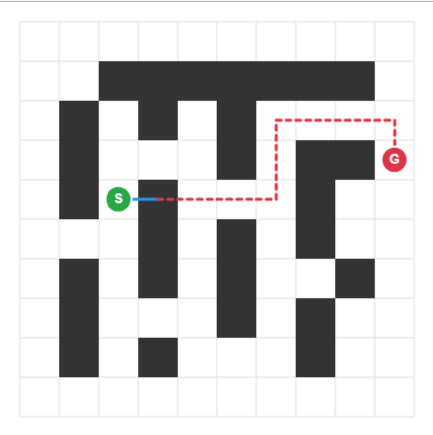
## Diagram: Grid-Based Pathfinding Visualization
### Overview
The image displays a 10x10 grid-based maze or pathfinding problem. It visually represents a computed path from a starting point to a goal point, navigating around static obstacles. The diagram is a technical illustration, likely used to demonstrate the output of a pathfinding algorithm (e.g., A*, Dijkstra's) in a discrete, grid-world environment.
### Components/Axes
* **Grid Structure:** A 10x10 square grid. Each cell is defined by light gray borders.
* **Cell States:**
* **Passable Cells:** White squares.
* **Obstacle Cells:** Solid black squares.
* **Key Points:**
* **Start Point (S):** A green circle containing a white capital letter "S". Positioned at grid coordinates (Row 5, Column 3), counting from the top-left as (1,1).
* **Goal Point (G):** A red circle containing a white capital letter "G". Positioned at grid coordinates (Row 4, Column 10).
* **Path:** A red dashed line connecting the Start and Goal points, indicating the computed route.
### Detailed Analysis
**1. Obstacle Map (Black Cells):**
The black cells form a complex barrier pattern. Their positions (using (Row, Column) from top-left) are:
* Row 2: Columns 3, 4, 5, 6, 7, 8, 9
* Row 3: Columns 2, 5, 8
* Row 4: Columns 2, 5, 8
* Row 5: Columns 4, 8
* Row 6: Columns 2, 4, 8
* Row 7: Columns 2, 4, 8, 10
* Row 8: Columns 2, 4, 8, 9
* Row 9: Columns 2, 4, 8
**2. Path Trajectory (Red Dashed Line):**
The path originates from the center of the green "S" circle and terminates at the center of the red "G" circle. Its route, described segment by segment:
* **Segment 1:** Moves horizontally **right** from (5,3) to (5,4). This is a short, solid blue line segment, distinct from the red dashes, possibly indicating the initial move or a different algorithm phase.
* **Segment 2:** From (5,4), the red dashed line begins, moving **right** to (5,5).
* **Segment 3:** Turns and moves **up** to (4,5).
* **Segment 4:** Turns and moves **right** to (4,6).
* **Segment 5:** Turns and moves **down** to (5,6).
* **Segment 6:** Turns and moves **right** to (5,7).
* **Segment 7:** Turns and moves **up** to (4,7).
* **Segment 8:** Turns and moves **right** to (4,8). *Note: This cell (4,8) is a black obstacle. The path appears to go *around* it, not through it. The line visually passes above the obstacle cell, suggesting the path's waypoints are at cell centers, and the line is drawn between them, skirting the edge of the obstacle.*
* **Segment 9:** From the vicinity of (4,8), the path moves **right** to (4,9).
* **Segment 10:** Finally, moves **right** to the Goal at (4,10).
**3. Spatial Relationships:**
* The Start (S) is located in a relatively open area on the left side of the grid.
* The Goal (G) is located on the far right edge.
* The path must navigate a central corridor formed by vertical black columns at columns 2, 4, 5, and 8. The chosen route threads through the gap between the obstacles at columns 5 and 8.
### Key Observations
* **Path Validity:** The path successfully connects S to G without passing through any black obstacle cells. It represents a valid, collision-free route.
* **Path Optimality:** The path is not a straight line (which is blocked) nor the shortest possible Manhattan distance path. It includes a detour (moving up to row 4, then down to row 5, then back up to row 4) to navigate around the central obstacle cluster. This suggests it may be the shortest *unblocked* path, or the result of a specific algorithm's cost function.
* **Visual Encoding:** The use of a distinct blue segment for the first move is notable. It could signify the initial step taken by an agent, a different cost, or simply a rendering artifact.
* **Obstacle Density:** The obstacles are concentrated in the central and upper-left regions, creating a bottleneck that the path must circumvent.
### Interpretation
This diagram is a classic representation of a **pathfinding solution in a grid world**. It demonstrates the core challenge of autonomous navigation: finding a viable route from an origin to a destination in an environment with barriers.
* **What it demonstrates:** The algorithm has successfully analyzed the spatial constraints (the black obstacles) and computed a sequence of discrete moves (right, up, right, etc.) that achieves the goal. The red dashed line is the visual proof of this solution.
* **Relationship between elements:** The Start and Goal define the problem's endpoints. The black cells define the problem's constraints. The red path is the solution that satisfies the constraints to connect the endpoints. The grid provides the discrete state space for the problem.
* **Underlying Logic:** The path's shape reveals the algorithm's logic. It doesn't take the most direct route but instead makes strategic turns to exploit gaps in the obstacle field. The detour through row 4 is necessary to pass between the vertical barriers at columns 5 and 8. This is characteristic of algorithms like A* which use heuristics to guide search towards the goal while avoiding explored dead ends.
* **Potential Context:** Such visualizations are fundamental in robotics (for mobile robot navigation), video game AI (for character pathing), and computational geometry. This specific instance could be a test case for comparing different pathfinding algorithms' efficiency and path quality.