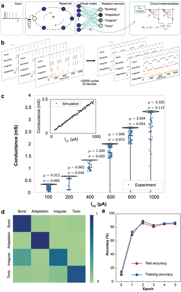
## Neural Network Analysis: Reservoir Computing and Accuracy Evaluation ### Overview The image presents a comprehensive analysis of a neural network implementation, likely a reservoir computing system. It includes a schematic of the network architecture, simulated and experimental conductance measurements, a confusion matrix, and training/testing accuracy plots. ### Components/Axes **Panel a: Network Architecture Diagram** * **Input:** A time-series input signal, represented as a series of pulses. * **Reservoir:** A recurrent neural network with interconnected nodes. A delay element labeled "τ" is present. * **Virtual Nodes:** Nodes connecting the reservoir to the readout neurons. * **Readout Neurons:** Four output neurons labeled "Bursting", "Adaptation", "Irregular", and "Tonic". * **Circuit Implementation:** A schematic showing the physical implementation of a weight (W_ij) as proportional to the difference between two conductances (G⁺ and G^-), controlled by a current I_CC. **Panel b: Spiking Activity** * Raster plots showing the spiking activity of the four readout neurons ("Tonic", "Bursting", "Irregular", "Adaptation") over time (0 to 1000 ms). * The data represents approximately 20,000 cycles across 25 devices. **Panel c: Conductance vs. Current (I_CC)** * **Y-axis:** Conductance (mS), ranging from 0 to 4. * **X-axis:** I_CC (μA), ranging from 0 to 1000. * **Inset:** Simulation data showing a positive correlation between I_CC and conductance. * **Main Plot:** Experimental data showing conductance values at discrete I_CC levels (100, 200, 400, 600, 800, 1000 μA). Each data point represents an individual measurement. Mean (μ) and standard deviation (σ) are indicated for each I_CC level. * I_CC = 100 μA: μ ≈ 0.312 mS, σ ≈ 0.060 mS * I_CC = 200 μA: μ ≈ 0.662 mS, σ ≈ 0.040 mS * I_CC = 400 μA: μ ≈ 1.330 mS, σ ≈ 0.033 mS * I_CC = 600 μA: μ ≈ 1.986 mS, σ ≈ 0.074 mS * I_CC = 800 μA: μ ≈ 2.658 mS, σ ≈ 0.084 mS * I_CC = 1000 μA: μ ≈ 3.325 mS, σ ≈ 0.112 mS **Panel d: Confusion Matrix** * A 4x4 confusion matrix showing the classification accuracy for the four neuron types ("Burst", "Adaptation", "Irregular", "Tonic"). * The color intensity represents the classification accuracy, ranging from 0 to 1. * The diagonal elements (true positives) are darker blue, indicating higher accuracy. **Panel e: Accuracy vs. Epoch** * **Y-axis:** Accuracy (%), ranging from 0 to 100. * **X-axis:** Epoch, ranging from 0 to 5. * **Test Accuracy:** Red line with square markers. * **Training Accuracy:** Blue line with circle markers. * Both lines show a rapid increase in accuracy from epoch 0 to epoch 2, followed by a plateau. ### Detailed Analysis **Panel a: Network Architecture** The diagram illustrates a reservoir computing architecture. The input signal is fed into a reservoir, which is a fixed, randomly connected recurrent neural network. The reservoir transforms the input into a higher-dimensional space. The readout neurons are trained to map the reservoir's state to the desired output. The circuit implementation shows how the weights between the reservoir and readout neurons are physically realized using conductances. **Panel b: Spiking Activity** The raster plots show the temporal dynamics of the readout neurons. Each plot represents the spiking activity of a single neuron type over time. The plots show the different firing patterns of the four neuron types. **Panel c: Conductance vs. Current (I_CC)** The inset plot shows the simulated relationship between I_CC and conductance, which is approximately linear. The main plot shows the experimental data, which exhibits variability around the mean values. The standard deviation increases with I_CC, indicating greater variability at higher current levels. **Panel d: Confusion Matrix** The confusion matrix shows the classification performance of the network. The diagonal elements represent the percentage of correctly classified instances for each neuron type. The off-diagonal elements represent the percentage of misclassified instances. The matrix suggests that some neuron types are more easily confused than others. **Panel e: Accuracy vs. Epoch** The plot shows the training and testing accuracy as a function of the number of training epochs. Both curves show a rapid increase in accuracy during the first two epochs, followed by a plateau. This indicates that the network learns quickly and reaches a stable performance level. The test accuracy is slightly lower than the training accuracy, which is expected due to overfitting. ### Key Observations * The reservoir computing system is capable of classifying different neuron types based on their spiking activity. * The conductance of the physical devices can be controlled by the current I_CC. * The classification accuracy reaches a high level after a few training epochs. * There is some variability in the conductance measurements, which may affect the performance of the network. ### Interpretation The data suggests that the reservoir computing system is a promising approach for implementing neural networks in hardware. The system is capable of learning complex patterns and achieving high classification accuracy. The physical implementation of the weights using conductances is a key advantage of this approach. The variability in the conductance measurements is a potential limitation that needs to be addressed in future work. The confusion matrix highlights potential areas for improvement in the classification performance. The accuracy plot demonstrates the learning capability of the system and the importance of training the readout neurons.