## Circuit Diagram: Programmable Device Architecture
### Overview
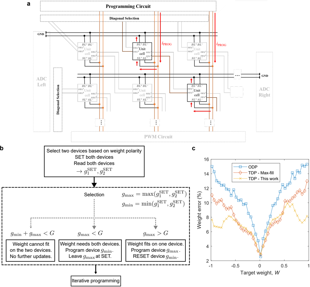
The diagram illustrates a programmable circuit architecture with diagonal selection, unit cells, and analog-to-digital converters (ADC). It includes a programming circuit, diagonal selection logic, and a PWM circuit.
### Components/Axes
- **Top Section**:
- **Programming Circuit**: Contains labeled unit cells (e.g., "BL", "BL'", "SEL", "SEL'") with bidirectional current paths (red arrows labeled *I_PROG*).
- **Diagonal Selection**: Connects unit cells via orange lines, with labels like "BL-BL'", "SEL-SEL'".
- **ADC Left/Right**: Grounded (GND) and connected to unit cells via black lines.
- **Bottom Section**:
- **PWM Circuit**: Grounded and linked to unit cells via black lines.
### Detailed Analysis
- **Unit Cells**: Each cell has labeled terminals (e.g., "BL", "BL'", "SEL", "SEL'") with bidirectional current flow.
- **Connections**: Diagonal selection paths (orange) link unit cells across rows.
- **Current Flow**: Red arrows (*I_PROG*) indicate programming current direction.
### Key Observations
- Symmetrical design with mirrored ADC left/right sections.
- Diagonal selection enables cross-row connectivity between unit cells.
---
## Flowchart: Iterative Programming Algorithm
### Overview
The flowchart outlines an iterative programming method for device selection and weight adjustment.
### Components/Axes
1. **Initial Step**:
- **Select two devices based on weight polarity**.
- **SET both devices** and **read both devices** to compute $ g_1^{SET}, g_2^{SET} $.
2. **Selection Logic**:
- $ g_{max} = \max(g_1^{SET}, g_2^{SET}) $, $ g_{min} = \min(g_1^{SET}, g_2^{SET}) $.
- Three conditional branches:
- **Weight cannot fit**: $ g_{min} + g_{max} < G $ → No further updates.
- **Weight needs both devices**: $ g_{max} < G $ → Leave $ g_{max} $ at SET.
- **Weight fits on one device**: $ g_{max} > G $ → Reset $ g_{min} $.
3. **Iterative Programming**: Loop back to device selection.
### Key Observations
- Conditional logic adapts based on weight polarity and magnitude.
- Emphasizes iterative optimization of device states.
---
## Line Graph: Weight Error vs. Target Weight
### Overview
The graph compares weight error (%) for three methods (ODP, TDP - Max-fill, TDP - This work) across target weights $ W \in [-1, 1] $.
### Components/Axes
- **X-axis**: Target weight $ W $ (range: -1 to 1).
- **Y-axis**: Weight error (%) (range: 0 to 16%).
- **Legend**:
- **ODP**: Blue squares (lowest error).
- **TDP - Max-fill**: Red diamonds (moderate error).
- **TDP - This work**: Yellow triangles (highest error).
### Detailed Analysis
- **Trends**:
- All methods show a V-shaped error curve with minima near $ W = 0 $.
- **ODP** consistently has the lowest error (e.g., ~2% at $ W = 0 $).
- **TDP - This work** exhibits the highest error (e.g., ~14% at $ W = 0 $).
- **Notable Outliers**:
- TDP - This work shows a sharp peak at $ W = 0.5 $ (~12% error).
### Key Observations
- ODP outperforms other methods across all $ W $.
- TDP - This work has significantly higher errors, suggesting suboptimal performance.
---
## Interpretation
1. **Circuit and Algorithm Synergy**:
- The programmable circuit (a) enables dynamic device selection via diagonal paths, while the flowchart (b) formalizes the iterative logic for optimizing device states.
- The PWM circuit likely modulates current for precise weight adjustments.
2. **Graph Insights**:
- **ODP’s Efficiency**: Its low error suggests superior weight precision, possibly due to optimized device selection.
- **TDP - This work’s Limitations**: Higher errors may stem from less effective programming strategies (e.g., suboptimal $ g_{min} $ resets).
3. **Practical Implications**:
- ODP is ideal for applications requiring minimal weight error.
- TDP - This work may need refinement for real-world deployment.
4. **Unresolved Questions**:
- Why does TDP - This work underperform? Is it due to algorithmic constraints or hardware limitations?
- How does diagonal selection impact error rates compared to other architectures?