## Diagram: Mathematical/Computational Mapping Relationships
### Overview
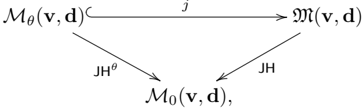
The diagram illustrates a structured relationship between three mathematical/computational entities:
1. **M_θ(v, d)** (top-left node)
2. **M(v, d)** (top-right node)
3. **M_0(v, d)** (bottom-center node)
Arrows represent transformations or mappings between these entities, labeled with symbolic operations. The structure suggests a hierarchical or dependency-based relationship.
---
### Components/Axes
- **Nodes**:
- **M_θ(v, d)**: Parameterized mapping with variables `v` (likely input vectors) and `d` (possibly dimensions or depth).
- **M(v, d)**: Simplified or derived version of `M_θ`.
- **M_0(v, d)**: Base or foundational mapping.
- **Arrows**:
- **j**: Maps `M_θ(v, d)` → `M(v, d)`. Likely a projection, simplification, or lossy transformation.
- **JH^θ**: Maps `M_θ(v, d)` → `M_0(v, d)`. Subscript `θ` implies parameterized homomorphism or function.
- **JH**: Maps `M(v, d)` → `M_0(v, d)`. Non-parameterized version of `JH^θ`.
- **Legend/Annotations**:
- No explicit legend, but arrow labels (`j`, `JH^θ`, `JH`) are directly annotated on edges.
---
### Detailed Analysis
1. **M_θ(v, d)** is the starting point, connected to both `M(v, d)` and `M_0(v, d)`.
2. **j** acts as a direct bridge between `M_θ` and `M`, suggesting a dependency or derivation.
3. **JH^θ** and **JH** represent two pathways to reach `M_0`:
- **JH^θ** preserves parameterization (`θ`), implying a specialized transformation.
- **JH** is a generalized version, stripping away `θ`-specific details.
---
### Key Observations
- **Commutativity**: The diagram implies that applying `j` followed by `JH` to `M_θ` should yield the same result as applying `JH^θ` directly. This is a common property in algebraic structures (e.g., category theory).
- **Hierarchy**: `M_θ` is the most specialized, `M` is intermediate, and `M_0` is the base abstraction.
- **Symmetry**: Both `M_θ` and `M` converge on `M_0`, suggesting `M_0` is a shared target or invariant.
---
### Interpretation
This diagram likely represents a **commutative diagram** in a mathematical framework (e.g., category theory, linear algebra, or machine learning). The mappings (`j`, `JH`, `JH^θ`) could correspond to:
- **Dimensionality reduction** (e.g., `j` as a projection).
- **Regularization** (e.g., `JH^θ` enforcing constraints via `θ`).
- **Abstraction layers** in a computational model, where `M_0` is a foundational component reused across contexts.
The parameterization (`θ`) in `JH^θ` suggests adaptability, while `JH` represents a fixed, universal mapping. The absence of numerical values implies this is a theoretical or architectural diagram rather than empirical data.
**Critical Insight**: The diagram emphasizes **modularity**—`M_θ` and `M` can be independently transformed into `M_0`, enabling reuse or composition in larger systems.