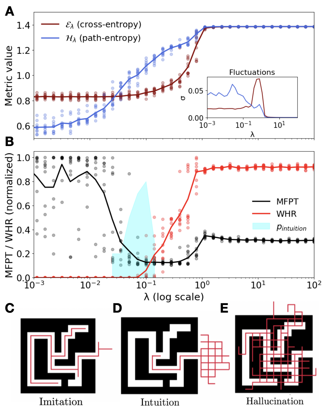
## Chart and Diagram Composite: Analysis of Pathfinding Metrics and Strategies ### Overview This image is a composite figure consisting of two line charts (A and B) and three illustrative diagrams (C, D, E). The charts display various metric values and normalized pathfinding performance against a parameter 'λ' on a logarithmic scale. The diagrams visually represent different pathfinding strategies—Imitation, Intuition, and Hallucination—within a maze-like environment. The overall figure appears to illustrate how different pathfinding behaviors emerge or are characterized across a range of 'λ' values. ### Components/Axes **Panel A: Metric Values vs. λ** * **Type**: Line chart with scatter points. * **X-axis**: Implicitly 'λ' (log scale), ranging from approximately $10^{-3}$ to $10^2$. Tick marks are at $10^{-3}, 10^{-2}, 10^{-1}, 10^0, 10^1, 10^2$. * **Y-axis**: "Metric value", ranging from 0.6 to 1.4. Tick marks are at 0.6, 0.8, 1.0, 1.2, 1.4. * **Legend (Top-left, inside chart area)**: * Brown line and scatter points: "$\mathcal{E}_\lambda$ (cross-entropy)" * Blue line and scatter points: "$H_\lambda$ (path-entropy)" * **Inset Chart (Top-right, inside Panel A)**: * **Title**: "Fluctuations" * **X-axis**: "λ", ranging from $10^{-3}$ to $10^2$. Tick marks are at $10^{-3}, 10^{-1}, 10^1$. * **Y-axis**: "σ", ranging from 0.00 to 0.05. Tick marks are at 0.00, 0.05. * **Data Series**: Brown line (corresponding to $\mathcal{E}_\lambda$) and Blue line (corresponding to $H_\lambda$). **Panel B: Normalized Performance Metrics vs. λ** * **Type**: Line chart with scatter points and a shaded area. * **X-axis**: "λ (log scale)", ranging from approximately $10^{-3}$ to $10^2$. Tick marks are at $10^{-3}, 10^{-2}, 10^{-1}, 10^0, 10^1, 10^2$. * **Y-axis**: "MFPT / WHR (normalized)", ranging from 0.0 to 1.0. Tick marks are at 0.0, 0.2, 0.4, 0.6, 0.8, 1.0. * **Legend (Top-right, inside chart area)**: * Black line and scatter points: "MFPT" * Red line and scatter points: "WHR" * Light cyan shaded area: "$p_{intuition}$" **Panels C, D, E: Illustrative Diagrams** * **Type**: Maze diagrams with overlaid paths. Each diagram shows a black background representing walls and white paths representing open space. Red lines indicate a trajectory or path. * **Panel C (Bottom-left)**: * **Title**: "Imitation" * **Content**: A simple maze with a single, direct red path following the white open space. * **Panel D (Bottom-center)**: * **Title**: "Intuition" * **Content**: A slightly more complex maze. A red path starts within the maze, follows a segment of the white path, and then extends outside the maze structure into a grid-like pattern of red lines. * **Panel E (Bottom-right)**: * **Title**: "Hallucination" * **Content**: A complex maze. Red paths are extensively overlaid both within the white open spaces and over the black wall areas, forming a dense, grid-like network that does not strictly adhere to the maze's navigable paths. ### Detailed Analysis **Panel A: Metric Values** * **$\mathcal{E}_\lambda$ (cross-entropy) - Brown Line**: * **Trend**: Starts relatively flat around a "Metric value" of 0.82 for λ from $10^{-3}$ to approximately $10^{-1.5}$. It then begins to increase sharply, crossing 1.0 around λ = $10^{-1}$, and continues to rise steeply to reach a plateau at approximately 1.38 for λ values greater than about $10^0$. * **Scatter Points**: Show some variability, especially in the rising phase, but generally follow the trend line. * **$H_\lambda$ (path-entropy) - Blue Line**: * **Trend**: Starts around a "Metric value" of 0.6 for λ from $10^{-3}$ to approximately $10^{-2}$. It then gradually increases, crossing 0.8 around λ = $10^{-1.5}$, and continues to rise, crossing 1.0 around λ = $10^{-1}$. It then rises more steeply, reaching a plateau at approximately 1.38 for λ values greater than about $10^0$. * **Scatter Points**: Show more variability than the brown line at lower λ values, but converge to the trend line at higher λ values. * **Comparison**: Both metrics increase with λ, eventually plateauing at a similar high value. $H_\lambda$ starts lower and increases earlier than $\mathcal{E}_\lambda$. They converge around λ = $10^0$ and then plateau together. * **Inset Chart: Fluctuations (σ)**: * **Brown Line (for $\mathcal{E}_\lambda$)**: Shows a low fluctuation (near 0.00) for λ < $10^{-1.5}$, then a sharp peak around λ = $10^{-0.5}$ (approximately 0.045), and then drops back to near 0.00 for λ > $10^0$. * **Blue Line (for $H_\lambda$)**: Shows a moderate fluctuation (around 0.02-0.03) for λ < $10^{-1}$, then decreases to near 0.00 for λ > $10^0$. It has a slight peak around λ = $10^{-1.5}$ (approx 0.035) before decreasing. **Panel B: Normalized Performance Metrics** * **MFPT (Mean First Passage Time) - Black Line**: * **Trend**: Starts high, around 0.9-1.0, for λ from $10^{-3}$ to $10^{-2}$. It then decreases sharply, reaching a minimum around 0.1-0.2 for λ between $10^{-1}$ and $10^0$. After this minimum, it increases slightly to plateau around 0.3-0.4 for λ values greater than $10^0$. * **Scatter Points**: Show significant variability, especially at lower λ values, but generally follow the trend line. * **WHR (Weighted Hitting Rate) - Red Line**: * **Trend**: Starts very low, near 0.0, for λ from $10^{-3}$ to approximately $10^{-1.5}$. It then increases sharply, crossing 0.2 around λ = $10^{-1}$, and continues to rise steeply to reach a plateau around 0.9-0.95 for λ values greater than about $10^0$. * **Scatter Points**: Show some variability, particularly in the rising phase, but generally follow the trend line. * **$p_{intuition}$ (Intuition Probability) - Light Cyan Shaded Area**: * **Distribution**: This area is low for λ < $10^{-1.5}$, then rises to a peak around λ = $10^{-1}$ to $10^{-0.5}$, where it covers a significant range of normalized values (from approx 0.0 to 0.8). It then decreases and is negligible for λ > $10^0$. This area broadly overlaps with the region where MFPT is decreasing and WHR is increasing. **Panels C, D, E: Illustrative Diagrams** * **C: Imitation**: The red path perfectly traces the navigable white path within the maze, suggesting a direct, known, or learned route. * **D: Intuition**: The red path follows the navigable white path for a segment, but then extends beyond the maze's physical boundaries into a structured, grid-like pattern. This suggests a process that starts with known information but then extrapolates or generates possibilities beyond the immediate environment. * **E: Hallucination**: The red paths are dense and chaotic, covering both navigable white paths and non-navigable black wall areas. This indicates a process that generates many paths without strict adherence to environmental constraints, potentially representing an overactive or unconstrained generation of possibilities. ### Key Observations * **Phase Transitions**: Both charts A and B show distinct phases or transitions as λ increases. * In Panel A, both entropy metrics are low and stable, then rise, and finally plateau. * In Panel B, MFPT starts high and drops, while WHR starts low and rises, both eventually plateauing. * **Inverse Relationship**: MFPT and WHR in Panel B exhibit an inverse relationship: as one decreases, the other increases, particularly in the range of λ from $10^{-2}$ to $10^0$. * **Intuition Zone**: The $p_{intuition}$ shaded area in Panel B peaks in the region where MFPT is at its minimum and WHR is rapidly increasing, suggesting that "intuition" is most prevalent when pathfinding efficiency (low MFPT) and success rate (high WHR) are transitioning. This also corresponds to the region where the fluctuations in $\mathcal{E}_\lambda$ are highest (Panel A inset). * **Entropy Behavior**: Path-entropy ($H_\lambda$) starts lower and increases earlier than cross-entropy ($\mathcal{E}_\lambda$), suggesting that the diversity of paths (path-entropy) might increase before the "error" or divergence from a target distribution (cross-entropy) becomes significant. * **Diagrammatic Correspondence**: The diagrams C, D, E visually represent distinct pathfinding strategies that likely correspond to different ranges of λ, though this correspondence is not explicitly mapped on the charts. "Imitation" might correspond to low λ, "Intuition" to intermediate λ (where $p_{intuition}$ is high), and "Hallucination" to high λ. ### Interpretation The data presented in this composite figure likely explores the behavior of a pathfinding or decision-making model as a parameter 'λ' is varied. 'λ' appears to control a trade-off or a transition between different modes of operation. * **Low λ (e.g., $10^{-3}$ to $10^{-2}$)**: In this regime, $\mathcal{E}_\lambda$ and $H_\lambda$ are low and stable, suggesting a predictable or constrained path generation process. MFPT is high, and WHR is low, indicating poor performance in finding paths. This could correspond to the "Imitation" strategy (Panel C), where the agent strictly follows known paths, which might be inefficient or fail in complex scenarios. The low fluctuations in entropy metrics further support a stable, perhaps rigid, behavior. * **Intermediate λ (e.g., $10^{-2}$ to $10^0$)**: This is a critical transition zone. * Both $\mathcal{E}_\lambda$ and $H_\lambda$ are rapidly increasing, indicating a greater diversity of paths and potentially a divergence from a simple, known distribution. * MFPT drops significantly, and WHR rises sharply, suggesting improved pathfinding efficiency and success. * Crucially, the $p_{intuition}$ area peaks here, and the fluctuations in $\mathcal{E}_\lambda$ are highest. This suggests that "Intuition" (Panel D) is a strategy characterized by exploring beyond immediate constraints, leading to better performance but also higher variability or uncertainty in the underlying process. The path extending outside the maze in Panel D visually supports this idea of extrapolation or generation beyond the given environment. * **High λ (e.g., $10^0$ to $10^2$)**: In this regime, both $\mathcal{E}_\lambda$ and $H_\lambda$ plateau at high values, indicating a high diversity of generated paths and a significant divergence from a baseline. MFPT slightly increases from its minimum, and WHR plateaus at a high value, suggesting good but not necessarily optimal performance. The "Hallucination" strategy (Panel E) could correspond to this phase, where the path generation process is overly unconstrained, creating many paths even through walls. While this might ensure finding a path (high WHR), the process itself is inefficient or "noisy" (higher MFPT than the minimum, high entropy values). In essence, the figure illustrates a model that transitions from a rigid, imitative behavior at low 'λ' to a more exploratory, "intuitive" phase at intermediate 'λ' (which optimizes performance), and finally to an overly generative, "hallucinatory" phase at high 'λ'. The parameter 'λ' likely tunes the balance between adherence to known information and the generation of novel possibilities. The peak in fluctuations for cross-entropy during the "intuitive" phase suggests that this optimal balance comes with inherent uncertainty or exploration.