## Diagram: Foundation Model - MLP Probe
### Overview
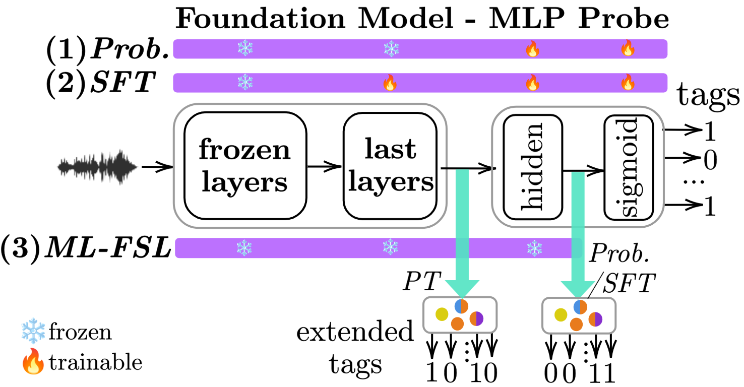
The image is a technical schematic illustrating three distinct training and probing strategies for a Foundation Model using an MLP (Multi-Layer Perceptron) probe. It visualizes the "frozen" versus "trainable" status of model components across three methods: (1) Prob., (2) SFT, and (3) ML-FSL. The diagram also details the architectural flow of the model, from input processing to the generation of standard and extended tags.
### Components/Axes
**Legend (Bottom-Left):**
* ❄️ (Snowflake icon): Represents "frozen" components (non-trainable).
* 🔥 (Fire icon): Represents "trainable" components.
**Rows (Top-Left):**
* **(1) Prob.:** Represents the Probing method.
* **(2) SFT:** Represents Supervised Fine-Tuning.
* **(3) ML-FSL:** Represents Multi-Label Few-Shot Learning.
**Architecture Flow (Center):**
* **Input:** An audio waveform icon.
* **Processing Blocks:**
* "frozen layers" (enclosed in a rounded rectangle).
* "last layers" (enclosed in a rounded rectangle).
* "hidden" (enclosed in a second rounded rectangle).
* "sigmoid" (enclosed in a second rounded rectangle).
* **Outputs:**
* "tags" (labeled on the right, with arrows pointing to 1, 0, ... 1).
* "extended tags" (labeled on the bottom-left of the lower section).
### Detailed Analysis
#### 1. Training/Probing Configurations
The three rows indicate the status of the model layers using the legend icons:
* **(1) Prob.:**
* Configuration: ❄️, ❄️, 🔥, 🔥.
* Status: The first two segments are frozen; the last two are trainable.
* **(2) SFT:**
* Configuration: ❄️, 🔥, 🔥, 🔥.
* Status: The first segment is frozen; the subsequent three are trainable.
* **(3) ML-FSL:**
* Configuration: ❄️, ❄️, ❄️.
* Status: All three segments are frozen.
#### 2. Architectural Flow and Extended Tags
The central diagram shows data flowing from left to right:
* **Main Path:** Input (waveform) → "frozen layers" → "last layers" → "hidden" → "sigmoid" → "tags".
* **Extended Tags Path:**
* Two cyan arrows point downward from the main flow.
* **First Arrow (Left):** Originates from the output of "last layers". Points to a box labeled **PT** (Pre-training).
* Inside the box: Four colored circles (yellow, orange, blue, purple).
* Output: "1 0 : 1 0".
* **Second Arrow (Right):** Originates from the output of "hidden". Points to a box labeled **Prob./SFT**.
* Inside the box: Four colored circles (yellow, blue, orange, purple).
* Output: "0 0 : 1 1".
### Key Observations
* **Gradient of Trainability:** There is a clear progression in the number of trainable parameters. ML-FSL is the most restrictive (entirely frozen), while SFT is the least restrictive (mostly trainable).
* **Information Extraction Points:** The "extended tags" are derived from different depths of the model. The "PT" tags are extracted earlier (after "last layers"), while the "Prob./SFT" tags are extracted later (after the "hidden" layer).
* **Binary Output:** Both the standard "tags" and the "extended tags" output binary sequences, suggesting a classification task.
### Interpretation
This diagram serves as a comparative architectural guide for adapting foundation models to downstream tasks.
* **Methodological Distinction:** The diagram contrasts how much of the foundation model is modified during adaptation. "Prob." (Probing) and "SFT" (Supervised Fine-Tuning) allow for parameter updates (fire icons), whereas "ML-FSL" (Multi-Label Few-Shot Learning) keeps the model entirely frozen, likely relying on the model's pre-existing representations without modification.
* **Feature Extraction:** The use of cyan arrows indicates that the "extended tags" are auxiliary outputs. By extracting features from different layers ("last layers" vs. "hidden"), the system likely captures different levels of abstraction—lower-level features for the "PT" (Pre-training) task and higher-level, more processed features for the "Prob./SFT" task.
* **Peircean Investigative Insight:** The visual language suggests a hierarchy of complexity. The "frozen" layers represent the immutable foundation, while the "trainable" layers represent the adaptive interface. The diagram implies that for few-shot learning (ML-FSL), the model is treated as a static feature extractor, whereas for SFT, the model is treated as a dynamic, tunable system.