## Chart/Diagram Type: Multi-Panel Figure
### Overview
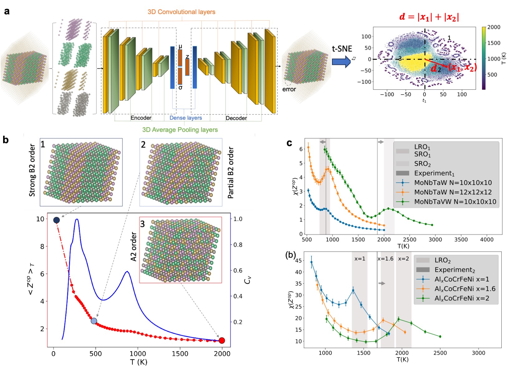
The image presents a multi-panel figure (a, b, c) exploring material properties and computational modeling. Panel (a) illustrates a 3D convolutional neural network architecture used for material analysis, along with a t-SNE projection. Panel (b) shows atomic structures representing different ordering states and a plot of <Zop>T and Cv vs. T. Panel (c) displays plots of χ(Zop) vs. T for different material compositions.
### Components/Axes
**Panel a:**
* **Diagram:** A schematic of a 3D Convolutional Neural Network.
* **Layers:** 3D Convolutional layers, 3D Average Pooling layers, Encoder, Dense layers (with labels μ, z, σ), Decoder.
* **Input:** A 3D representation of a material structure.
* **Output:** An "error" signal and a t-SNE projection.
* **t-SNE Plot:**
* **Axes:** t1 (x-axis), t2 (y-axis). Both range from approximately -100 to 100.
* **Color Scale:** Temperature (T) in Kelvin, ranging from 500 (blue) to 2000 (yellow).
* **Equation:** d = |x1| + |x2|
* **Annotation:** d2 = (x1, x2)
**Panel b:**
* **Atomic Structures:**
* Structure 1: "Strong B2 order"
* Structure 2: "Partial B2 order"
* Structure 3: "A2 order" (enclosed in a red box)
* **Plot:**
* **Left Y-axis:** <Zop>T, ranging from 0 to 10.
* **Right Y-axis:** Cv, ranging from 0 to 1.0.
* **X-axis:** T (K), ranging from 0 to 2000.
* **Data Series:**
* <Zop>T: Red line with circular markers.
* Cv: Blue line.
**Panel c:**
* **Top Plot:**
* **Y-axis:** χ(Zop), ranging from 0 to 6.
* **X-axis:** T (K), ranging from 500 to 4000.
* **Data Series:**
* MoNbTaW N=10x10x10: Blue line with error bars.
* MoNbTaW N=12x12x12: Orange line with error bars.
* MoNbTaVW N=10x10x10: Green line with error bars.
* **Vertical Shaded Regions:** Gray, indicating LRO1, SRO1, and SRO2.
* **Legend:** Located at the top-right.
* **Bottom Plot:**
* **Y-axis:** χ(Zop), ranging from 5 to 45.
* **X-axis:** T (K), ranging from 800 to 3000.
* **Data Series:**
* AlxCoCrFeNi x=1: Blue line with error bars.
* AlxCoCrFeNi x=1.6: Orange line with error bars.
* AlxCoCrFeNi x=2: Green line with error bars.
* **Vertical Shaded Regions:** Gray, indicating LRO2.
* **Labels:** x=1, x=1.6, x=2 are marked on the plot.
* **Legend:** Located at the top-right.
### Detailed Analysis or ### Content Details
**Panel a:**
* The 3D convolutional neural network takes a 3D material structure as input.
* The network consists of convolutional layers, pooling layers, and dense layers.
* The output is used to generate a t-SNE projection, which visualizes the high-dimensional data in a 2D space.
* The t-SNE plot shows clusters of points, colored by temperature.
**Panel b:**
* The atomic structures represent different degrees of ordering in the material.
* Structure 1 (Strong B2 order) shows a high degree of order.
* Structure 2 (Partial B2 order) shows a partial degree of order.
* Structure 3 (A2 order) shows a disordered state.
* The <Zop>T curve (red) shows a peak around T = 200 K, then decreases as temperature increases.
* At T = 0 K, <Zop>T is approximately 9.5.
* At T = 500 K, <Zop>T is approximately 2.5.
* At T = 2000 K, <Zop>T is approximately 1.
* The Cv curve (blue) shows a sharp peak around T = 200 K, then decreases and shows a smaller peak around T = 750 K.
**Panel c:**
* **Top Plot:**
* The blue line (MoNbTaW N=10x10x10) starts at approximately χ(Zop) = 3.2 at T = 500 K, decreases to a minimum around T = 1000 K, and then remains relatively flat.
* The orange line (MoNbTaW N=12x12x12) starts at approximately χ(Zop) = 4.0 at T = 500 K, decreases to a minimum around T = 1250 K, and then increases slightly.
* The green line (MoNbTaVW N=10x10x10) starts at approximately χ(Zop) = 5.8 at T = 500 K, decreases to a minimum around T = 1250 K, and then increases.
* **Bottom Plot:**
* The blue line (AlxCoCrFeNi x=1) starts at approximately χ(Zop) = 44 at T = 800 K, decreases to a minimum around T = 1500 K, and then increases slightly.
* The orange line (AlxCoCrFeNi x=1.6) starts at approximately χ(Zop) = 22 at T = 800 K, decreases to a minimum around T = 1500 K, and then increases slightly.
* The green line (AlxCoCrFeNi x=2) starts at approximately χ(Zop) = 32 at T = 800 K, decreases to a minimum around T = 1500 K, and then decreases slightly.
### Key Observations
* Panel (a) shows the architecture of a neural network used for material analysis.
* Panel (b) shows the relationship between atomic ordering and material properties.
* Panel (c) shows the temperature dependence of χ(Zop) for different material compositions.
* The t-SNE plot in panel (a) visualizes the high-dimensional data in a 2D space, revealing clusters of points corresponding to different temperatures.
* The <Zop>T and Cv curves in panel (b) show peaks around T = 200 K, indicating a phase transition.
* The χ(Zop) curves in panel (c) show minima around T = 1000-1500 K, indicating a change in material properties.
### Interpretation
The data suggests that the neural network is capable of capturing the complex relationships between atomic structure, temperature, and material properties. The t-SNE plot provides a visual representation of the high-dimensional data, revealing clusters of points corresponding to different temperatures. The <Zop>T, Cv, and χ(Zop) curves provide quantitative information about the temperature dependence of material properties. The observed peaks and minima in these curves indicate phase transitions and changes in material behavior. The different material compositions exhibit distinct behaviors, highlighting the importance of composition in determining material properties. The vertical shaded regions in panel (c) likely indicate regions of different ordering types.