TECHNICAL ASSET FINGERPRINT
90eef10fe595db45dbb06cc5
Click to view fullscreen
Press ESC or click to close
FOUND IN PAPERS
EXPERT: healer-alpha-free VERSION 1
RUNTIME: free/openrouter/healer-alpha
INTEL_VERIFIED
### Multi-Panel Scientific Figure: 3D Convolutional Autoencoder for Alloy Structural Analysis
#### **Overview**
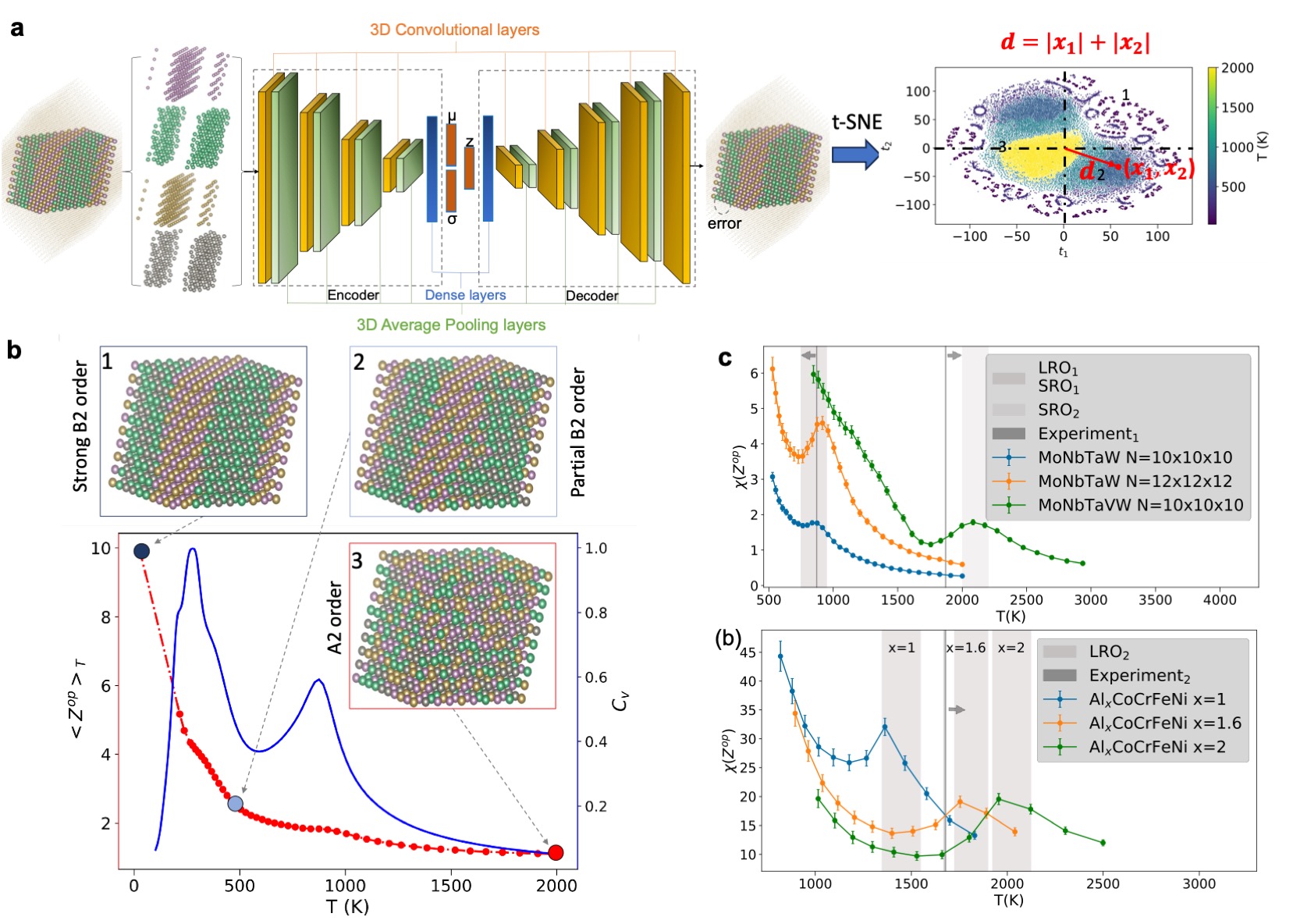
The image is a multi-panel (a, b, c) scientific figure illustrating a **3D convolutional autoencoder** applied to analyze atomic structures of alloys, with temperature-dependent properties and latent space visualization. It combines machine learning (autoencoder architecture) with materials science (alloy ordering, temperature effects).
### **Panel (a): 3D Convolutional Autoencoder & t-SNE Latent Space**
#### **Components/Axes**
- **Left (Input):** 3D atomic structures (colored atoms, likely different elements) and a set of 3D atomic configurations (colored clusters: green, purple, brown, gray).
- **Middle (Autoencoder Architecture):**
- *Encoder:* 3D Convolutional layers → Dense layers (with latent variables \( \mu, \sigma, z \)).
- *Decoder:* 3D Convolutional layers → 3D Average Pooling layers.
- Labels: *“3D Convolutional layers”*, *“Encoder”*, *“Dense layers”*, *“Decoder”*, *“3D Average Pooling layers”*.
- **Right (t-SNE Plot):**
- Axes: \( t_1 \) (x-axis, -100 to 100), \( t_2 \) (y-axis, -100 to 100).
- Color bar: Temperature \( T(\text{K}) \) (500 K = blue, 2000 K = yellow).
- Formula: \( d = |x_1| + |x_2| \); red arrow: \( d_2(x_1, x_2) \).
- Labeled points: 1, 2, 3 (clustered regions).
#### **Detailed Analysis**
The autoencoder processes atomic configurations, compresses them to a latent space (\( z \)), and reconstructs them. The t-SNE plot visualizes the latent space:
- **Yellow cluster (center):** High temperature (\( \sim 2000 \, \text{K} \)).
- **Blue/purple clusters (periphery):** Lower temperatures (\( \sim 500–1500 \, \text{K} \)).
This shows temperature-dependent organization of structural features in the latent space.
#### **Key Observations**
- Latent space clusters correlate with temperature (high \( T \) = central yellow, low \( T \) = peripheral blue/purple).
- The autoencoder uses 3D convolutions to capture spatial atomic relationships.
#### **Interpretation**
The autoencoder captures temperature-dependent structural features in the latent space, enabling visualization of how atomic order (e.g., B2, A2) relates to temperature. This links machine learning to materials science by quantifying structural changes.
### **Panel (b): Atomic Order & Temperature-Dependent Properties**
#### **Components/Axes**
- **Top (Atomic Structures):**
- 1: *“Strong B2 order”* (ordered atomic arrangement).
- 2: *“Partial B2 order”* (partially disordered).
- **Bottom (Plot):**
- X-axis: \( T(\text{K}) \) (0 to 2000).
- Left Y-axis: \( \langle Z^{\text{op}} \rangle \) (order parameter, 0 to 10).
- Right Y-axis: \( C_v \) (heat capacity, 0 to 1.0).
- Data: Red dots (with error bars) for \( \langle Z^{\text{op}} \rangle \); blue line for \( C_v \).
- Atomic structures: 1 (Strong B2), 2 (Partial B2), 3 (A2 order, *“A2 order”*) with dashed lines to the plot.
#### **Detailed Analysis**
- \( \langle Z^{\text{op}} \rangle \) (red dots) **decreases with \( T \)**: ~10 at 0 K → ~1 at 2000 K (loss of order).
- \( C_v \) (blue line) has **peaks** (likely phase transitions).
- Atomic structures show increasing disorder: *Strong B2* → *Partial B2* → *A2* (with \( T \)).
#### **Key Observations**
- \( \langle Z^{\text{op}} \rangle \) (order parameter) quantifies structural order, decreasing with \( T \).
- \( C_v \) peaks suggest thermal phase transitions.
- Atomic structures visually confirm increasing disorder with \( T \).
#### **Interpretation**
The plot links atomic order (B2, A2) to temperature: \( \langle Z^{\text{op}} \rangle \) quantifies order, and \( C_v \) indicates thermal properties. The autoencoder (panel a) likely captures these structural changes in its latent space.
### **Panel (c): Temperature-Dependent Susceptibility (\( \chi(Z^{\text{op}}) \)) for Alloys**
#### **Components/Axes**
- **Top Plot:**
- X-axis: \( T(\text{K}) \) (500 to 4000).
- Y-axis: \( \chi(Z^{\text{op}}) \) (susceptibility, 0 to 6).
- Legend: *“LRO₁”*, *“SRO₁”*, *“SRO₂”*, *“Experiment₁”* (gray shaded regions); data series:
- MoNbTaW \( N=10 \times 10 \times 10 \) (blue),
- MoNbTaW \( N=12 \times 12 \times 12 \) (orange),
- MoNbTaVW \( N=10 \times 10 \times 10 \) (green).
- **Bottom Plot:**
- X-axis: \( T(\text{K}) \) (1000 to 3000).
- Y-axis: \( \chi(Z^{\text{op}}) \) (10 to 45).
- Legend: *“LRO₂”*, *“Experiment₂”* (gray shaded regions); data series:
- \( \text{Al}_x\text{CoCrFeNi} \, x=1 \) (blue),
- \( \text{Al}_x\text{CoCrFeNi} \, x=1.6 \) (orange),
- \( \text{Al}_x\text{CoCrFeNi} \, x=2 \) (green).
#### **Detailed Analysis**
- **Top Plot:** \( \chi(Z^{\text{op}}) \) **decreases with \( T \)** for all series. MoNbTaVW (green) has higher \( \chi \) than MoNbTaW (blue/orange). Gray regions (LRO₁, SRO₁, SRO₂, Experiment₁) mark long/short-range order regimes.
- **Bottom Plot:** \( \chi(Z^{\text{op}}) \) **decreases with \( T \)**. \( \text{Al}_x\text{CoCrFeNi} \, x=1 \) (blue) has higher \( \chi \) than \( x=1.6 \) (orange) and \( x=2 \) (green). Gray regions (LRO₂, Experiment₂) mark order regimes.
#### **Key Observations**
- \( \chi(Z^{\text{op}}) \) (susceptibility) decreases with \( T \), indicating reduced order.
- Alloy composition (MoNbTaW vs MoNbTaVW; \( \text{Al}_x\text{CoCrFeNi} \, x=1 \) vs 1.6 vs 2) affects \( \chi \).
- Gray regions mark order-disorder transitions (LRO = long-range order, SRO = short-range order).
#### **Interpretation**
The plots show how alloy composition and temperature affect structural order (via \( \chi(Z^{\text{op}}) \)), with long/short-range order regimes. The autoencoder’s latent space (panel a) likely correlates with these order parameters, enabling predictive modeling of alloy behavior.
### **Cross-Panel Interpretation**
The figure integrates machine learning (autoencoder) with materials science to:
1. Capture temperature-dependent structural features in a latent space (panel a).
2. Quantify atomic order and thermal properties (panel b).
3. Analyze alloy composition and temperature effects on order (panel c).
This workflow enables predictive modeling of alloy behavior, linking structural changes to temperature and composition.
**Note:** All text is in English; no other language is present. Values are approximate (e.g., temperature ranges, \( \chi \) magnitudes) based on visual analysis.
DECODING INTELLIGENCE...