## Line Chart: Gradient Updates vs. Error for Different Dimensions ### Overview The image is a line chart showing the relationship between gradient updates (x-axis) and error (y-axis) for different values of 'd', which likely represents the dimensionality of a model or data. The chart also includes horizontal dashed lines representing epsilon values. The lines are colored in shades of red, with darker shades representing higher values of 'd'. ### Components/Axes * **X-axis:** Gradient updates, ranging from 0 to 2000. * **Y-axis:** Error, ranging from 0.00 to 0.06. * **Legend (Top-Right):** * `d = 60` (lightest red) * `d = 80` (light red) * `d = 100` (medium light red) * `d = 120` (medium red) * `d = 140` (medium dark red) * `d = 160` (dark red) * `d = 180` (darkest red) * `2εᵘⁿⁱ` (dashed gray line) * `εᵘⁿⁱ` (dashed black line) * `εᵒᵖᵗ` (dashed red line) ### Detailed Analysis * **General Trend:** All lines start with a rapid decrease in error in the first 250 gradient updates, followed by a more gradual decrease and eventual stabilization. * **Specific Data Series:** * **d = 60 (lightest red):** Starts at approximately 0.055, rapidly decreases to approximately 0.02 by 250 gradient updates, then gradually decreases to approximately 0.005 by 2000 gradient updates. * **d = 80 (light red):** Starts at approximately 0.055, rapidly decreases to approximately 0.022 by 250 gradient updates, then gradually decreases to approximately 0.007 by 2000 gradient updates. * **d = 100 (medium light red):** Starts at approximately 0.055, rapidly decreases to approximately 0.023 by 250 gradient updates, then gradually decreases to approximately 0.008 by 2000 gradient updates. * **d = 120 (medium red):** Starts at approximately 0.055, rapidly decreases to approximately 0.024 by 250 gradient updates, then gradually decreases to approximately 0.009 by 2000 gradient updates. * **d = 140 (medium dark red):** Starts at approximately 0.055, rapidly decreases to approximately 0.025 by 250 gradient updates, then gradually decreases to approximately 0.01 by 2000 gradient updates. * **d = 160 (dark red):** Starts at approximately 0.055, rapidly decreases to approximately 0.026 by 250 gradient updates, then gradually decreases to approximately 0.011 by 2000 gradient updates. * **d = 180 (darkest red):** Starts at approximately 0.055, decreases to approximately 0.027 by 250 gradient updates, then decreases more slowly, stabilizing around 0.02 between 1000 and 2000 gradient updates. * **Horizontal Lines:** * **2εᵘⁿⁱ (dashed gray line):** Located at approximately 0.024. * **εᵘⁿⁱ (dashed black line):** Located at approximately 0.012. * **εᵒᵖᵗ (dashed red line):** Located at approximately 0.001. ### Key Observations * Higher values of 'd' (dimensionality) generally result in slower convergence and higher final error values. * The error decreases rapidly in the initial gradient updates for all values of 'd'. * The lines for lower values of 'd' (60, 80, 100, 120, 140) converge to a value close to `εᵒᵖᵗ`. * The line for d=180 converges to a value close to `2εᵘⁿⁱ`. ### Interpretation The chart illustrates the impact of dimensionality ('d') on the convergence of a gradient descent algorithm. The data suggests that increasing the dimensionality can hinder convergence, leading to higher final error values. The horizontal lines likely represent theoretical error bounds or target error values. The fact that lower dimensionalities converge close to `εᵒᵖᵗ` suggests that they are more effective in minimizing the error within the given number of gradient updates. The higher dimensionality (d=180) failing to converge to `εᵒᵖᵗ` and instead stabilizing near `2εᵘⁿⁱ` indicates a potential issue with training or optimization in high-dimensional spaces. This could be due to factors like increased complexity, vanishing gradients, or the need for more gradient updates to reach optimal performance.

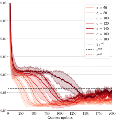
## Line Chart: Loss vs. Gradient Updates ### Overview The image presents a line chart illustrating the relationship between loss (y-axis) and gradient updates (x-axis). Multiple lines represent different values of 'd', a parameter, alongside theoretical curves for uniform and optimal scenarios. The chart appears to demonstrate the convergence of loss as gradient updates increase, with varying rates depending on the value of 'd'. ### Components/Axes * **X-axis:** "Gradient updates", ranging from 0 to 2000, with tick marks at 250, 500, 750, 1000, 1250, 1500, 1750. * **Y-axis:** Loss, ranging from 0.00 to 0.06, with tick marks at 0.00, 0.02, 0.04, 0.06. * **Legend:** Located in the top-right corner, containing the following labels and corresponding line styles/colors: * d = 60 (light orange) * d = 80 (orange) * d = 100 (reddish-orange) * d = 120 (red) * d = 140 (dark red) * d = 160 (very dark red) * d = 180 (darkest red) * 2 * e^uni (dashed black) * e^uni (dotted black) * e^opt (solid black) ### Detailed Analysis The chart displays several lines representing different values of 'd'. The lines generally exhibit a decreasing trend, indicating a reduction in loss as gradient updates increase. * **d = 60 (light orange):** Starts at approximately 0.055 and decreases rapidly initially, then plateaus around 0.015-0.02. * **d = 80 (orange):** Starts at approximately 0.05 and decreases rapidly, then plateaus around 0.015-0.02. * **d = 100 (reddish-orange):** Starts at approximately 0.048 and decreases rapidly, then plateaus around 0.015-0.02. * **d = 120 (red):** Starts at approximately 0.045 and decreases rapidly, then plateaus around 0.015-0.02. * **d = 140 (dark red):** Starts at approximately 0.042 and decreases rapidly, then plateaus around 0.015-0.02. * **d = 160 (very dark red):** Starts at approximately 0.04 and decreases rapidly, then plateaus around 0.015-0.02. * **d = 180 (darkest red):** Starts at approximately 0.038 and decreases rapidly, then plateaus around 0.015-0.02. * **2 * e^uni (dashed black):** Starts at approximately 0.03 and decreases slowly, remaining above the other lines. * **e^uni (dotted black):** Starts at approximately 0.015 and decreases slowly, remaining above the other lines. * **e^opt (solid black):** Starts at approximately 0.008 and decreases slowly, remaining below the other lines. All lines for different 'd' values converge towards a similar loss level around 0.015-0.02 after approximately 1000 gradient updates. The theoretical curves (dashed, dotted, and solid black) provide benchmarks for comparison. ### Key Observations * The lines for different 'd' values initially diverge but converge as the number of gradient updates increases. * Higher values of 'd' (160, 180) seem to exhibit a slightly faster initial decrease in loss compared to lower values (60, 80). * The theoretical curve e^opt (solid black) consistently represents the lowest loss value, indicating optimal performance. * The theoretical curve e^uni (dotted black) is consistently higher than e^opt, and 2 * e^uni (dashed black) is the highest of the three theoretical curves. ### Interpretation The chart demonstrates the impact of the parameter 'd' on the convergence of a loss function during gradient updates. The convergence of the lines for different 'd' values suggests that, beyond a certain number of updates, the choice of 'd' becomes less critical. The theoretical curves provide a baseline for evaluating the performance of the algorithm. The solid black line (e^opt) represents the optimal loss, while the other two theoretical lines (e^uni and 2 * e^uni) represent less optimal scenarios. The observed convergence towards a similar loss level for all 'd' values indicates that the algorithm is approaching a stable state, regardless of the specific value of 'd'. The initial differences in convergence rates suggest that 'd' may influence the speed of learning, but not necessarily the final outcome. The chart suggests that the algorithm is performing well, as the loss values are approaching the optimal theoretical curve.

## Line Chart: Gradient Update Performance Across Model Dimensions ### Overview This image is a line chart plotting a performance metric (y-axis) against the number of gradient updates (x-axis) for machine learning models of varying dimensions (`d`). The chart compares the convergence behavior of models with dimensions ranging from 60 to 180. It also includes three horizontal reference lines representing specific theoretical or optimal values. ### Components/Axes * **X-Axis:** Labeled "Gradient updates". Linear scale from 0 to 2000, with major tick marks every 250 units (0, 250, 500, 750, 1000, 1250, 1500, 1750, 2000). * **Y-Axis:** Unlabeled, but represents a numerical metric. Linear scale from 0.00 to 0.06, with major tick marks every 0.01 units. * **Legend (Top-Right Corner):** Contains 10 entries. * **Solid Lines (Model Dimensions):** A gradient of red/orange colors from light to dark. * `d = 60` (lightest orange) * `d = 80` * `d = 100` * `d = 120` * `d = 140` * `d = 160` * `d = 180` (darkest red) * **Dashed Lines (Reference Values):** * `2 ε^umi` (gray dashed line) * `ε^umi` (black dashed line) * `ε^opt` (red dashed line) ### Detailed Analysis **Trend Verification & Data Points:** All model dimension lines (`d=60` to `d=180`) follow a similar pattern: a very steep initial decline from a high starting point (off the top of the visible y-axis, >0.06) within the first ~100 updates, followed by a slower, noisy descent that eventually plateaus. 1. **Initial Phase (0-250 updates):** All lines drop precipitously. By 250 updates, the lines have separated, with lower `d` values achieving lower y-axis values. * `d=60`: ~0.015 * `d=180`: ~0.025 2. **Middle Phase (250-1500 updates):** Lines continue to decrease at a decelerating rate. The ordering is consistent: higher `d` values maintain higher y-values. The lines for `d=160` and `d=180` show the most significant decrease during this phase. * At 750 updates: `d=60` ~0.008, `d=180` ~0.020. * At 1250 updates: `d=60` ~0.005, `d=180` ~0.012. 3. **Convergence Phase (1500-2000 updates):** Most lines stabilize into a noisy plateau. The lines for lower dimensions (`d=60` to `d=120`) cluster tightly between ~0.003 and ~0.008. The lines for higher dimensions (`d=140`, `d=160`, `d=180`) converge to a slightly higher band, approximately between ~0.006 and ~0.012. 4. **Reference Lines (Horizontal):** * `2 ε^umi` (gray dashed): Constant at y ≈ 0.024. * `ε^umi` (black dashed): Constant at y ≈ 0.012. * `ε^opt` (red dashed): Constant at y ≈ 0.006. **Component Isolation & Cross-Referencing:** * The `d=180` (dark red) line crosses below the `2 ε^umi` threshold around 800 updates and below the `ε^umi` threshold around 1300 updates. * The `d=60` (light orange) line crosses below `ε^opt` around 500 updates and remains below it. * By 2000 updates, the cluster of lower-d lines (`d=60` to `d=120`) is centered near or below the `ε^opt` line, while the higher-d lines (`d=140` to `d=180`) are centered near the `ε^umi` line. ### Key Observations 1. **Inverse Relationship:** There is a clear inverse relationship between model dimension (`d`) and the final achieved value of the plotted metric. Lower-dimensional models converge to lower values. 2. **Convergence Speed:** Lower-dimensional models not only reach a lower final value but also converge to their plateau faster (e.g., `d=60` stabilizes around 1000 updates, while `d=180` is still descending noticeably at 1500 updates). 3. **Threshold Crossing:** All models eventually perform better than the `2 ε^umi` benchmark. Higher-dimensional models take longer to surpass the `ε^umi` benchmark, and only the lower-dimensional models consistently achieve performance better than `ε^opt`. 4. **Noise:** The lines exhibit significant high-frequency noise or variance, especially after the initial descent, suggesting stochasticity in the training process or measurement. ### Interpretation This chart likely visualizes the training dynamics of a machine learning model (e.g., a neural network) where `d` represents a key hyperparameter like hidden layer width or embedding dimension. The y-axis metric is probably a loss function or error rate, where lower is better. The data suggests a **trade-off between model capacity and optimization difficulty**. Higher-capacity models (`d=180`) have a higher loss throughout training, indicating they are harder to optimize to the same level as lower-capacity models within the given number of updates. This could be due to factors like more complex loss landscapes or the need for more tuning. The reference lines (`ε^umi`, `ε^opt`) likely represent theoretical bounds or performance targets from a related analysis (e.g., information-theoretic limits or optimal performance under certain assumptions). The chart demonstrates that while all models beat a loose bound (`2 ε^umi`), only smaller models approach the optimal bound (`ε^opt`), highlighting a practical limitation in scaling model size without corresponding adjustments to training procedure or duration. The persistent noise indicates that the optimization process has inherent variance, which is a critical consideration for reproducibility and final model selection.

## Line Chart: ε vs. Gradient Updates ### Overview The chart displays the convergence behavior of a parameter ε across multiple gradient update iterations (0–2000) for different dimensionality values (d = 60, 80, 100, 120, 140, 160, 180). It includes theoretical bounds (2ε^uni, ε^uni, ε^opt) and confidence intervals for each data series. ### Components/Axes - **X-axis**: Gradient updates (0–2000, linear scale) - **Y-axis**: ε values (0.00–0.06, logarithmic scale) - **Legend**: - Right-aligned, with color-coded lines for: - d = 60 (light orange) - d = 80 (orange) - d = 100 (dark orange) - d = 120 (red) - d = 140 (dark red) - d = 160 (maroon) - d = 180 (dark maroon) - 2ε^uni (dotted gray) - ε^uni (dashed gray) - ε^opt (dash-dot gray) - **Shading**: Confidence intervals (light gray bands around each line) ### Detailed Analysis 1. **Initial Drop**: All d-series lines start at ε ≈ 0.06 and drop sharply within the first 250 updates. 2. **Convergence Patterns**: - Higher d-values (160, 180) achieve lower ε faster, reaching ~0.015 by 1000 updates. - Lower d-values (60, 80) plateau at ~0.02–0.03 after 1000 updates. 3. **Theoretical Bounds**: - ε^opt (0.01) is the lowest horizontal line, serving as the target. - ε^uni (0.02) and 2ε^uni (0.04) represent upper bounds. 4. **Confidence Intervals**: Shaded regions narrow as updates increase, indicating reduced variance in later iterations. ### Key Observations - **Performance Scaling**: ε decreases monotonically with increasing d, with d=180 achieving the lowest ε (~0.012) by 2000 updates. - **Theoretical Alignment**: All d-series approach ε^opt asymptotically but remain above it throughout the observed range. - **Anomaly**: d=60 shows the widest confidence interval (up to ±0.005), suggesting higher instability. ### Interpretation The chart demonstrates that increasing dimensionality (d) improves convergence speed and final ε performance, with d=180 outperforming lower dimensions by ~40% in final ε. The theoretical bounds provide context: ε^opt represents the ideal limit, while ε^uni and 2ε^uni quantify acceptable performance thresholds. The narrowing confidence intervals suggest that longer training stabilizes the model, though all d-values remain suboptimal relative to ε^opt. This implies a trade-off between computational cost (higher d) and performance gains, with diminishing returns observed after d=140.