# Technical Document Extraction: Comparison of Neural Network Architectures
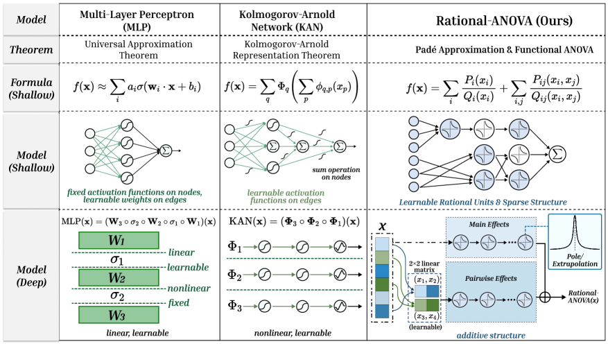
This document provides a comprehensive extraction of the data and structural comparisons presented in the provided image. The image is a technical table comparing three neural network models: **Multi-Layer Perceptron (MLP)**, **Kolmogorov-Arnold Network (KAN)**, and the proposed **Rational-ANOVA**.
---
## 1. High-Level Table Structure
The information is organized into a grid with five functional rows and three model columns.
| Row Category | Column 1: Multi-Layer Perceptron (MLP) | Column 2: Kolmogorov-Arnold Network (KAN) | Column 3: Rational-ANOVA (Ours) |
| :--- | :--- | :--- | :--- |
| **Model** | Multi-Layer Perceptron (MLP) | Kolmogorov-Arnold Network (KAN) | Rational-ANOVA (Ours) |
| **Theorem** | Universal Approximation Theorem | Kolmogorov-Arnold Representation Theorem | Padé Approximation & Functional ANOVA |
| **Formula (Shallow)** | $f(\mathbf{x}) \approx \sum_{i} a_i \sigma(\mathbf{w}_i \cdot \mathbf{x} + b_i)$ | $f(\mathbf{x}) = \sum_{q} \Phi_q \left( \sum_{p} \phi_{q,p}(x_p) \right)$ | $f(\mathbf{x}) = \sum_{i} \frac{P_i(x_i)}{Q_i(x_i)} + \sum_{i,j} \frac{P_{ij}(x_i, x_j)}{Q_{ij}(x_i, x_j)}$ |
| **Model (Shallow)** | Diagram of fixed activations on nodes | Diagram of learnable activations on edges | Diagram of learnable rational units |
| **Model (Deep)** | Stacked linear/nonlinear layers | Composition of nonlinear functions | Additive structure with Main/Pairwise effects |
---
## 2. Detailed Component Analysis
### Column 1: Multi-Layer Perceptron (MLP)
* **Theorem:** Relies on the **Universal Approximation Theorem**.
* **Formula (Shallow):** Approximates a function as a weighted sum of nonlinear activations of linear combinations of inputs.
* **Model (Shallow) Diagram:**
* **Structure:** Input nodes connect to a hidden layer of four nodes, which then converge to a single summation ($\Sigma$) output node.
* **Key Characteristic:** Text states: *"fixed activation functions on nodes, learnable weights on edges"*.
* **Model (Deep) Diagram:**
* **Logic:** Represented as a composition of matrices and activations: $\text{MLP}(\mathbf{x}) = (\mathbf{W}_3 \circ \sigma_2 \circ \mathbf{W}_2 \circ \sigma_1 \circ \mathbf{W}_1)(\mathbf{x})$.
* **Visual Stack:** Alternating green blocks ($W_1, W_2, W_3$) and dashed lines ($\sigma_1, \sigma_2$).
* **Labels:** $W$ layers are labeled as **linear** and **learnable**. $\sigma$ layers are labeled as **nonlinear** and **fixed**.
### Column 2: Kolmogorov-Arnold Network (KAN)
* **Theorem:** Relies on the **Kolmogorov-Arnold Representation Theorem**.
* **Formula (Shallow):** A nested summation where the inner functions $\phi_{q,p}$ and outer functions $\Phi_q$ are univariate.
* **Model (Shallow) Diagram:**
* **Structure:** Input nodes connect via edges containing activation function symbols to summation nodes ($\Sigma$).
* **Key Characteristic:** Text states: *"learnable activation functions on edges"* and *"sum operation on nodes"*.
* **Model (Deep) Diagram:**
* **Logic:** Represented as a composition of function layers: $\text{KAN}(\mathbf{x}) = (\mathbf{\Phi}_3 \circ \mathbf{\Phi}_2 \circ \mathbf{\Phi}_1)(\mathbf{x})$.
* **Visual Flow:** Three parallel horizontal tracks ($\Phi_1, \Phi_2, \Phi_3$), each showing a sequence of three learnable activation nodes.
* **Labels:** The layers are described as **nonlinear** and **learnable**.
### Column 3: Rational-ANOVA (Ours)
* **Theorem:** Combines **Padé Approximation** and **Functional ANOVA**.
* **Formula (Shallow):** Expresses the function as a sum of univariate rational functions (Main Effects) and bivariate rational functions (Pairwise Effects).
* **Model (Shallow) Diagram:**
* **Structure:** Input nodes connect to blue-shaded "Rational Units" (depicting rational function curves). The structure is sparse, with some inputs skipping directly to specific units.
* **Key Characteristic:** Text states: *"Learnable Rational Units & Sparse Structure"*.
* **Model (Deep) Diagram:**
* **Input $\mathcal{X}$:** A vertical vector of features.
* **Main Effects Block:** Features pass into a sequence of rational units.
* **Pairwise Effects Block:** Features are grouped via a "$2 \times 2$ linear matrix (learnable)" to create pairs like $(x_1, x_2)$ and $(x_3, x_4)$, which then pass through rational units.
* **Pole/Extrapolation:** A call-out box shows a graph with a sharp peak, labeled *"Pole/Extrapolation"*, indicating the model's ability to handle rational singularities.
* **Output:** The Main and Pairwise effects are combined at a summation node ($\oplus$) to produce **Rational-ANOVA(x)**.
* **Labels:** The overall architecture is described as an **additive structure**.
---
## 3. Summary of Comparative Trends
1. **Parameter Location:** MLP places learnable parameters on edges (weights); KAN places them on edges (functions); Rational-ANOVA uses learnable rational units in a structured additive format.
2. **Function Type:** MLP uses fixed nonlinearities; KAN uses learnable univariate functions; Rational-ANOVA uses learnable rational functions (fractions of polynomials $P/Q$).
3. **Interpretability:** Rational-ANOVA explicitly separates "Main Effects" and "Pairwise Effects," following the Functional ANOVA decomposition, which is typically more interpretable than the dense connectivity of MLPs.