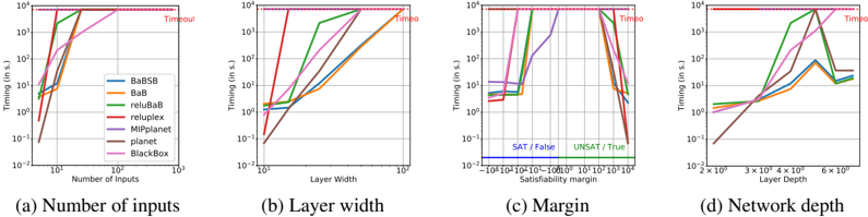
## Chart Type: Multiple Line Graphs ### Overview The image contains four line graphs comparing the timing performance (in seconds) of different verification methods (BaBSB, BaB, reluBaB, reluplex, MIPplanet, planet, and BlackBox) against varying parameters: number of inputs, layer width, satisfiability margin, and network depth. The y-axis (Timing) is displayed on a logarithmic scale. A horizontal line labeled "Timeout" is present at the top of each graph, indicating a maximum time limit. ### Components/Axes **General:** * **Y-axis (all graphs):** "Timing (in s.)" - Logarithmic scale from 10^-2 to 10^4. * **Legend (top-left of first graph):** * BaBSB (Blue) * BaB (Orange) * reluBaB (Green) * reluplex (Red) * MIPplanet (Purple) * planet (Brown) * BlackBox (Pink) * **Timeout Line:** A horizontal dotted red line at y = 10^4, labeled "Timeout" in red text. **Graph (a): Number of inputs** * **X-axis:** "Number of Inputs" - Linear scale from 10^0 to 10^3. **Graph (b): Layer width** * **X-axis:** "Layer Width" - Linear scale from 10^1 to 10^2. **Graph (c): Margin** * **X-axis:** "Satisfiability margin" - Logarithmic scale from -10^6 to 10^6. Labels "SAT / False" and "UNSAT / True" are present. **Graph (d): Network depth** * **X-axis:** "Layer Depth" - Linear scale from 2 x 10^0 to 6 x 10^0. ### Detailed Analysis **Graph (a): Number of inputs** * **BaBSB (Blue):** Relatively flat at approximately 10^-1 until around 10^1 inputs, then increases gradually to approximately 10^0 at 10^3 inputs. * **BaB (Orange):** Starts at approximately 10^-1 and increases to approximately 10^1 at 10^3 inputs. * **reluBaB (Green):** Increases sharply from approximately 10^0 to the timeout line (10^4) between 10^0 and 10^1 inputs. * **reluplex (Red):** Increases sharply from approximately 10^-1 to the timeout line (10^4) between 10^0 and 10^1 inputs. * **MIPplanet (Purple):** Increases sharply from approximately 10^-1 to approximately 10^3 between 10^0 and 10^1 inputs, then continues to increase to the timeout line (10^4) at 10^2 inputs. * **planet (Brown):** Starts at approximately 10^-1 and increases to approximately 10^0 at 10^3 inputs. * **BlackBox (Pink):** Increases sharply from approximately 10^-1 to the timeout line (10^4) between 10^0 and 10^1 inputs. **Graph (b): Layer width** * **BaBSB (Blue):** Relatively flat at approximately 10^-1. * **BaB (Orange):** Increases from approximately 10^-1 to approximately 10^2. * **reluBaB (Green):** Increases sharply from approximately 10^-1 to the timeout line (10^4) between 10^1 and 10^2 layer width. * **reluplex (Red):** Increases sharply from approximately 10^-2 to the timeout line (10^4) between 10^1 and 10^2 layer width. * **MIPplanet (Purple):** Increases sharply from approximately 10^-1 to the timeout line (10^4) between 10^1 and 10^2 layer width. * **planet (Brown):** Increases from approximately 10^-2 to approximately 10^1. * **BlackBox (Pink):** Increases sharply from approximately 10^-1 to the timeout line (10^4) between 10^1 and 10^2 layer width. **Graph (c): Margin** * **BaBSB (Blue):** Remains relatively constant at approximately 10^-2. * **BaB (Orange):** Remains relatively constant at approximately 10^0. * **reluBaB (Green):** Increases sharply from approximately 10^-1 to the timeout line (10^4) between -10^1 and -10^0 margin, then drops sharply to approximately 10^1 at 10^1 margin, and then decreases to approximately 10^0 at 10^6 margin. * **reluplex (Red):** Increases sharply from approximately 10^-1 to the timeout line (10^4) between -10^1 and -10^0 margin, then drops sharply to approximately 10^1 at 10^1 margin, and then decreases to approximately 10^0 at 10^6 margin. * **MIPplanet (Purple):** Increases sharply from approximately 10^-1 to approximately 10^3 between -10^1 and -10^0 margin, then drops sharply to approximately 10^1 at 10^1 margin, and then decreases to approximately 10^0 at 10^6 margin. * **planet (Brown):** Remains relatively constant at approximately 10^-1. * **BlackBox (Pink):** Increases sharply from approximately 10^-1 to the timeout line (10^4) between -10^1 and -10^0 margin, then drops sharply to approximately 10^1 at 10^1 margin, and then decreases to approximately 10^0 at 10^6 margin. **Graph (d): Network depth** * **BaBSB (Blue):** Increases from approximately 10^-1 to approximately 10^1. * **BaB (Orange):** Increases from approximately 10^0 to approximately 10^1. * **reluBaB (Green):** Increases sharply from approximately 10^0 to the timeout line (10^4) between 2x10^0 and 4x10^0 layer depth, then drops sharply to approximately 10^1 at 6x10^0 layer depth. * **reluplex (Red):** Increases sharply from approximately 10^-1 to the timeout line (10^4) between 2x10^0 and 4x10^0 layer depth, then drops sharply to approximately 10^1 at 6x10^0 layer depth. * **MIPplanet (Purple):** Increases sharply from approximately 10^-1 to approximately 10^3 between 2x10^0 and 4x10^0 layer depth, then drops sharply to approximately 10^1 at 6x10^0 layer depth. * **planet (Brown):** Increases from approximately 10^-1 to approximately 10^0. * **BlackBox (Pink):** Increases sharply from approximately 10^-1 to approximately 10^3 between 2x10^0 and 4x10^0 layer depth, then drops sharply to approximately 10^1 at 6x10^0 layer depth. ### Key Observations * The "reluBaB", "reluplex", "MIPplanet", and "BlackBox" methods frequently reach the timeout limit (10^4 seconds) as the number of inputs, layer width, and network depth increase, and as the satisfiability margin approaches the "UNSAT/True" region. * The "BaBSB", "BaB", and "planet" methods generally exhibit lower timing values and do not reach the timeout limit within the tested ranges. * The satisfiability margin graph (c) shows a sharp increase in timing for "reluBaB", "reluplex", "MIPplanet", and "BlackBox" as the margin transitions from negative to positive values, followed by a decrease as the margin increases further. ### Interpretation The graphs illustrate the performance of different verification methods under varying conditions. The "reluBaB", "reluplex", "MIPplanet", and "BlackBox" methods are more sensitive to increases in the number of inputs, layer width, and network depth, often exceeding the timeout limit. The satisfiability margin significantly impacts the timing of these methods, with a peak in computation time observed around the transition from "SAT/False" to "UNSAT/True". The "BaBSB", "BaB", and "planet" methods appear to be more scalable and robust, maintaining lower timing values across the tested parameter ranges. The data suggests that the choice of verification method should be carefully considered based on the specific characteristics of the neural network being analyzed.

\n ## Charts: Performance Timing vs. Various Parameters ### Overview The image presents four charts, each depicting the timing (in seconds) of different solvers (BaBSB, BaB, reluBaB, relupiex, MIPplanet, planet, BlackBox) as a function of varying parameters: (a) Number of Inputs, (b) Layer Width, (c) Satisfiability Margin, and (d) Network Depth. The y-axis of all charts is on a logarithmic scale. The charts appear to be evaluating the scalability and performance of these solvers under different problem characteristics. ### Components/Axes Each chart shares the following components: * **X-axis:** Represents the independent variable being tested (Number of Inputs, Layer Width, Satisfiability Margin, Network Depth). * **Y-axis:** Labeled "Timing (in s)" and is a logarithmic scale ranging from 10^-2 to 10¹. * **Legend:** Located in the top-left corner of each chart, identifying the different solvers by color. The solvers are: * BaBSB (Blue) * BaB (Orange) * reluBaB (Green) * relupiex (Red) * MIPplanet (Purple) * planet (Pink) * BlackBox (Brown) * **Title:** Each chart has a title indicating the parameter being varied. * **Annotations:** The charts include annotations like "Timeout" and "Time" indicating where solvers exceeded a time limit. ### Detailed Analysis or Content Details **Chart (a): Number of Inputs** * **X-axis:** Number of Inputs, ranging from approximately 10⁰ to 10⁴. * **Trends:** * BaBSB (Blue): Starts at approximately 0.01s and increases rapidly, reaching the timeout limit (10¹ s) around 10³ inputs. * BaB (Orange): Starts at approximately 0.01s and increases rapidly, reaching the timeout limit around 10³ inputs. * reluBaB (Green): Starts at approximately 0.01s and increases rapidly, reaching the timeout limit around 10³ inputs. * relupiex (Red): Starts at approximately 0.01s and increases rapidly, reaching the timeout limit around 10³ inputs. * MIPplanet (Purple): Starts at approximately 0.01s and increases rapidly, reaching the timeout limit around 10³ inputs. * planet (Pink): Starts at approximately 0.01s and increases rapidly, reaching the timeout limit around 10³ inputs. * BlackBox (Brown): Starts at approximately 0.01s and increases rapidly, reaching the timeout limit around 10³ inputs. **Chart (b): Layer Width** * **X-axis:** Layer Width, ranging from approximately 10^-2 to 10¹. * **Trends:** * BaBSB (Blue): Increases rapidly from approximately 0.01s to the timeout limit around a layer width of 10¹. * BaB (Orange): Increases rapidly from approximately 0.01s to the timeout limit around a layer width of 10¹. * reluBaB (Green): Increases rapidly from approximately 0.01s to the timeout limit around a layer width of 10¹. * relupiex (Red): Increases rapidly from approximately 0.01s to the timeout limit around a layer width of 10¹. * MIPplanet (Purple): Increases rapidly from approximately 0.01s to the timeout limit around a layer width of 10¹. * planet (Pink): Increases rapidly from approximately 0.01s to the timeout limit around a layer width of 10¹. * BlackBox (Brown): Increases rapidly from approximately 0.01s to the timeout limit around a layer width of 10¹. **Chart (c): Margin** * **X-axis:** Satisfiability Margin, ranging from approximately 10^-1 to 10¹. * **Trends:** * BaBSB (Blue): Remains relatively constant at approximately 0.01s until the margin reaches 10⁰, then increases to approximately 0.1s. * BaB (Orange): Remains relatively constant at approximately 0.01s until the margin reaches 10⁰, then increases to approximately 0.1s. * reluBaB (Green): Remains relatively constant at approximately 0.01s until the margin reaches 10⁰, then increases to approximately 0.1s. * relupiex (Red): Remains relatively constant at approximately 0.01s until the margin reaches 10⁰, then increases to approximately 0.1s. * MIPplanet (Purple): Remains relatively constant at approximately 0.01s until the margin reaches 10⁰, then increases to approximately 0.1s. * planet (Pink): Remains relatively constant at approximately 0.01s until the margin reaches 10⁰, then increases to approximately 0.1s. * BlackBox (Brown): Remains relatively constant at approximately 0.01s until the margin reaches 10⁰, then increases to approximately 0.1s. **Chart (d): Network Depth** * **X-axis:** Network Depth, ranging from approximately 2 x 10³ to 6 x 10³. * **Trends:** * BaBSB (Blue): Increases from approximately 0.01s to approximately 0.1s, then fluctuates. * BaB (Orange): Increases from approximately 0.01s to approximately 0.1s, then fluctuates. * reluBaB (Green): Increases from approximately 0.01s to approximately 1s. * relupiex (Red): Increases from approximately 0.01s to approximately 1s. * MIPplanet (Purple): Increases from approximately 0.01s to approximately 0.1s, then fluctuates. * planet (Pink): Increases from approximately 0.01s to approximately 1s. * BlackBox (Brown): Increases from approximately 0.01s to approximately 0.1s, then fluctuates. ### Key Observations * All solvers exhibit a rapid increase in timing as the Number of Inputs and Layer Width increase, quickly reaching the timeout limit. * The Satisfiability Margin has a relatively small impact on timing until it reaches a certain threshold, after which timing increases. * Network Depth shows more varied behavior, with some solvers (reluBaB, planet) exhibiting a significant increase in timing, while others (BaBSB, BaB, MIPplanet) show more moderate fluctuations. * The logarithmic y-axis emphasizes the exponential growth in timing for many solvers. ### Interpretation The data suggests that the performance of these solvers is highly sensitive to the size and complexity of the problem, as measured by the Number of Inputs and Layer Width. The rapid increase in timing indicates that these problems quickly become intractable for these solvers as these parameters grow. The Satisfiability Margin appears to have a threshold effect, where timing remains relatively constant until a certain margin is reached, after which performance degrades. The Network Depth results suggest that some solvers are more susceptible to the effects of increased network complexity than others. The consistent "Timeout" annotations across most solvers for larger values of Number of Inputs and Layer Width indicate a fundamental limitation in the scalability of these approaches. The differences in timing between solvers, even before reaching the timeout limit, suggest that some solvers are more efficient than others for certain problem characteristics. The varying responses to Network Depth suggest that the choice of solver should be tailored to the specific structure of the problem being solved. The logarithmic scale is crucial for understanding the magnitude of the performance differences, highlighting the exponential growth in computation time.

\n ## Multi-Plot Performance Analysis: Algorithm Timing vs. Problem Parameters ### Overview The image is a composite of four line charts (labeled a, b, c, d) comparing the execution timing (in seconds) of seven different algorithms or methods across varying problem parameters. All plots share a common y-axis ("Timing (in s)") on a logarithmic scale (10^-1 to 10^4) and a common red dashed horizontal line indicating a "Timeout" at 10^4 seconds. The plots analyze scalability with respect to the number of inputs, layer width, satisfiability margin, and network depth. ### Components/Axes * **Common Y-Axis:** Label: "Timing (in s)". Scale: Logarithmic, ranging from 10^-1 (0.1 s) to 10^4 (10,000 s). * **Common Timeout Line:** A red dashed horizontal line at y = 10^4 seconds, labeled "Timeout" in red text at the right end of each plot. * **Legend (Present in all plots, top-left):** Lists seven data series with corresponding colors: * BaBSB (Blue) * BaB (Orange) * BaB-ER (Green) * reluplex (Red) * MIPplanet (Purple) * Planet (Brown) * BlackBox (Pink) * **Subplot Titles/Captions (Below each plot):** * (a) Number of inputs * (b) Layer width * (c) Margin * (d) Network depth ### Detailed Analysis #### **Subplot (a): Number of inputs** * **X-Axis:** Label: "Number of inputs". Scale: Logarithmic, with major ticks at 10^0 (1), 10^1 (10), 10^2 (100), 10^3 (1000). * **Trends & Data Points:** * **General Trend:** All algorithms show increasing timing as the number of inputs grows. The increase is roughly linear on the log-log plot for most, suggesting a polynomial time complexity relationship. * **BaBSB (Blue):** Starts near 10^0 s for 1 input. Increases steadily, crossing 10^1 s around 10 inputs, 10^2 s around 100 inputs, and approaches but does not reach the timeout at 1000 inputs (~5x10^3 s). * **BaB (Orange):** Follows a very similar path to BaBSB, nearly overlapping it. * **BaB-ER (Green):** Starts slightly higher than BaBSB/BaB. Increases more steeply, crossing 10^2 s before 100 inputs and hitting the timeout line (10^4 s) at approximately 200-300 inputs. * **reluplex (Red):** Starts the lowest (~2x10^-1 s for 1 input). Increases very steeply, crossing all other lines and hitting the timeout at approximately 50-60 inputs. * **MIPplanet (Purple):** Starts around 10^0 s. Increases at a moderate rate, crossing 10^2 s around 100 inputs and hitting the timeout at approximately 500-600 inputs. * **Planet (Brown):** Starts near 10^0 s. Increases similarly to MIPplanet but slightly slower, hitting the timeout at approximately 800-900 inputs. * **BlackBox (Pink):** Starts the highest (~5x10^0 s for 1 input). Increases at the slowest rate, remaining below 10^2 s even at 1000 inputs. #### **Subplot (b): Layer width** * **X-Axis:** Label: "Layer Width". Scale: Logarithmic, with major ticks at 10^0 (1), 10^1 (10), 10^2 (100). * **Trends & Data Points:** * **General Trend:** Timing generally increases with layer width, but the scaling behavior varies significantly between algorithms. * **BaBSB (Blue) & BaB (Orange):** Show a relatively gentle increase. At width=1, timing is ~10^0 s. At width=100, timing is ~10^2 s. * **BaB-ER (Green):** Increases more sharply than BaBSB/BaB, hitting the timeout at a width of approximately 30-40. * **reluplex (Red):** Shows the steepest increase, hitting the timeout at a width of approximately 5-6. * **MIPplanet (Purple):** Increases steeply, hitting the timeout at a width of approximately 20-25. * **Planet (Brown):** Increases at a rate between BaBSB and MIPplanet, hitting the timeout at a width of approximately 50-60. * **BlackBox (Pink):** Shows a very gentle, almost flat increase, remaining around 10^1 s across the entire range of widths. #### **Subplot (c): Margin** * **X-Axis:** Label: "Satisfiability margin". Scale: Logarithmic, with major ticks at 10^-1 (0.1), 10^0 (1), 10^1 (10), 10^2 (100). * **Additional Annotations:** Text labels at the bottom: "SAT / False" (left of 10^0) and "UNSAT / True" (right of 10^0). * **Trends & Data Points:** * **General Trend:** This plot shows non-monotonic behavior. Timing often decreases as the margin increases from very small values (10^-1) to around 1 (the SAT/UNSAT boundary), then increases again for larger margins. * **BaBSB (Blue) & BaB (Orange):** Show a "U-shaped" curve. Minimum timing (~2-3x10^0 s) occurs near margin=1. Timing rises to ~10^2 s at both margin=0.1 and margin=100. * **BaB-ER (Green):** Similar U-shape but with higher overall timing. Minimum (~10^1 s) near margin=1. Hits timeout at margin=100. * **reluplex (Red):** Shows a very sharp V-shape. Minimum timing (~10^0 s) at margin=1. Increases extremely steeply on both sides, hitting timeout at margin=0.3 and margin=3. * **MIPplanet (Purple):** Shows a U-shape. Minimum (~10^1 s) near margin=1. Hits timeout at margin=100. * **Planet (Brown):** Shows a U-shape. Minimum (~10^1 s) near margin=1. Hits timeout at margin=100. * **BlackBox (Pink):** Shows a relatively flat, high timing (~10^2 s) across the entire margin range, with a slight dip near margin=1. #### **Subplot (d): Network depth** * **X-Axis:** Label: "Layer Depth". Scale: Linear, with major ticks at 2, 3, 4, 5, 6. * **Trends & Data Points:** * **General Trend:** Timing increases with network depth for all algorithms. The increase appears exponential (linear on the semi-log plot). * **BaBSB (Blue) & BaB (Orange):** Start at ~10^0 s for depth=2. Increase to ~10^2 s at depth=6. * **BaB-ER (Green):** Starts near BaBSB at depth=2. Increases more steeply, hitting timeout at depth=5. * **reluplex (Red):** Starts lowest at depth=2 (~2x10^-1 s). Increases the most steeply, hitting timeout at depth=4. * **MIPplanet (Purple):** Starts around 10^0 s at depth=2. Increases steeply, hitting timeout at depth=5. * **Planet (Brown):** Starts around 10^0 s at depth=2. Increases at a rate similar to MIPplanet, hitting timeout at depth=5. * **BlackBox (Pink):** Starts highest at depth=2 (~10^1 s). Increases at the slowest rate, reaching ~10^3 s at depth=6. ### Key Observations 1. **Performance Hierarchy:** reluplex is consistently the fastest for very small/simple problems (low inputs, narrow layers, margin=1, shallow depth) but scales the worst, hitting timeouts earliest. BlackBox is consistently the slowest for small problems but scales the best, often being the only algorithm not to timeout for large/complex instances. 2. **Critical Parameter:** The "Satisfiability margin" plot (c) reveals a critical performance sweet spot at margin=1 (the SAT/UNSAT boundary) for most algorithms, where timing is minimized. 3. **Scalability Trends:** BaBSB and BaB demonstrate the most robust and predictable polynomial scaling across inputs, width, and depth. BaB-ER, MIPplanet, and Planet show intermediate scaling, often hitting timeouts for large parameters. 4. **Timeout Clusters:** In plots (a), (b), and (d), algorithms tend to hit the timeout in a consistent order: reluplex first, followed by BaB-ER/MIPplanet/Planet, then BaBSB/BaB, with BlackBox often not timing out. ### Interpretation This composite chart provides a comprehensive scalability analysis of neural network verification or analysis algorithms. The data suggests a fundamental trade-off between raw speed on small instances and robustness to problem size. * **Algorithm Selection Guidance:** The choice of algorithm should be heavily informed by the expected problem scale. For quick checks on small networks, reluplex is optimal. For large-scale, industrial-sized networks, BlackBox, despite its high constant overhead, becomes the only viable option. BaBSB/BaB offer a balanced middle ground. * **Problem Difficulty Insight:** The pronounced minimum at margin=1 in plot (c) indicates that problems near the decision boundary (where the property is barely true or false) are computationally easiest for these solvers. Problems with large margins (clearly true or false) are harder, likely because they require exploring a larger search space to confirm the margin. * **Architectural Sensitivity:** The steep increases in plots (b) and (d) show that algorithm performance is highly sensitive to network architecture (width and depth). This implies that verifier-friendly network design (e.g., keeping layers narrow and shallow) is crucial for tractable analysis. * **Underlying Methods:** The performance profiles hint at the underlying methods. reluplex's steep scaling suggests a simplex-like method that struggles with dimensionality. BlackBox's flat scaling suggests a sampling or optimization-based approach with high overhead but good scalability. The BaB family (BaBSB, BaB, BaB-ER) likely uses branch-and-bound, with BaB-ER incorporating an extra refinement step that adds overhead but may improve precision.

## Line Graphs: Algorithm Performance Analysis ### Overview The image contains four line graphs (a-d) comparing the timing performance of seven algorithms (BaBSB, BaB, reluBaB, reluplex, MIPplanet, planet, BlackBox) across four parameters: number of inputs, layer width, satisfaction margin, and network depth. All graphs use a logarithmic scale for timing (y-axis) and linear/logarithmic scales for parameters (x-axis). A horizontal "Timeout" threshold line (10^4 s) is present in all graphs. ### Components/Axes 1. **Graph (a): Number of inputs** - X-axis: "Number of inputs" (10^1 to 10^3) - Y-axis: "Timing (in s.)" (10^-2 to 10^4) - Legend: Positioned top-right, colors match lines: - Blue: BaBSB - Orange: BaB - Green: reluBaB - Red: reluplex - Purple: MIPplanet - Brown: planet - Pink: BlackBox - Dashed red: Timeout threshold 2. **Graph (b): Layer width** - X-axis: "Layer width" (10^1 to 10^2) - Y-axis: "Timing (in s.)" (10^-2 to 10^4) - Legend: Same as (a), positioned top-right 3. **Graph (c): Satisfaction margin** - X-axis: "Satisfaction margin" (10^-4 to 10^4) - Y-axis: "Timing (in s.)" (10^-2 to 10^4) - Legend: Includes SAT/False (blue) and UNSAT/True (green) in addition to algorithm colors 4. **Graph (d): Network depth** - X-axis: "Layer depth" (2×10^0 to 6×10^0) - Y-axis: "Timing (in s.)" (10^-2 to 10^4) - Legend: Same as (a), positioned top-right ### Detailed Analysis #### Graph (a) Trends - **Timeout (red dashed)**: Flat line at 10^4 s (timeout threshold) - **BaBSB (blue)**: Sharp initial rise, plateaus at ~10^2 s - **BaB (orange)**: Steeper rise than BaBSB, plateaus at ~10^3 s - **reluBaB (green)**: Gradual rise, plateaus at ~10^2 s - **reluplex (red)**: Sharp rise, plateaus at ~10^3 s - **MIPplanet (purple)**: Moderate rise, plateaus at ~10^2 s - **planet (brown)**: Steep rise, plateaus at ~10^3 s - **BlackBox (pink)**: Gradual rise, plateaus at ~10^2 s #### Graph (b) Trends - **Timeout (red dashed)**: Flat line at 10^4 s - **BaBSB (blue)**: Gradual rise, plateaus at ~10^2 s - **BaB (orange)**: Steeper rise than BaBSB, plateaus at ~10^3 s - **reluBaB (green)**: Moderate rise, plateaus at ~10^2 s - **reluplex (red)**: Sharp rise, plateaus at ~10^3 s - **MIPplanet (purple)**: Gradual rise, plateaus at ~10^2 s - **planet (brown)**: Steep rise, plateaus at ~10^3 s - **BlackBox (pink)**: Moderate rise, plateaus at ~10^2 s #### Graph (c) Trends - **Timeout (red dashed)**: Flat line at 10^4 s - **SAT/False (blue)**: Flat line at ~10^-1 s - **UNSAT/True (green)**: Sharp rise at ~10^2 s, plateaus at 10^4 s - **BaBSB (blue)**: Gradual rise, plateaus at ~10^2 s - **BaB (orange)**: Steeper rise than BaBSB, plateaus at ~10^3 s - **reluBaB (green)**: Moderate rise, plateaus at ~10^2 s - **reluplex (red)**: Sharp rise, plateaus at ~10^3 s - **MIPplanet (purple)**: Gradual rise, plateaus at ~10^2 s - **planet (brown)**: Steep rise, plateaus at ~10^3 s - **BlackBox (pink)**: Moderate rise, plateaus at ~10^2 s #### Graph (d) Trends - **Timeout (red dashed)**: Flat line at 10^4 s - **BaBSB (blue)**: Gradual rise, plateaus at ~10^2 s - **BaB (orange)**: Steeper rise than BaBSB, plateaus at ~10^3 s - **reluBaB (green)**: Moderate rise, plateaus at ~10^2 s - **reluplex (red)**: Sharp rise, plateaus at ~10^3 s - **MIPplanet (purple)**: Gradual rise, plateaus at ~10^2 s - **planet (brown)**: Steep rise, plateaus at ~10^3 s - **BlackBox (pink)**: Moderate rise, plateaus at ~10^2 s ### Key Observations 1. **Timeout Consistency**: All algorithms hit the 10^4 s timeout threshold at maximum parameter values. 2. **Algorithm Sensitivity**: - **BaBSB/BlackBox**: Most stable across parameters, plateauing at ~10^2 s - **BaB/planet**: High sensitivity to layer width and network depth - **reluplex**: Most sensitive to satisfaction margin (sharp rise in graph c) 3. **Anomalies**: - **reluplex** shows a sharp drop in graph (d) at 4×10^0 layer depth - **UNSAT/True** (green) in graph (c) exhibits a discontinuous jump at 10^2 margin ### Interpretation The data suggests algorithm performance varies significantly with input complexity: - **BaBSB and BlackBox** demonstrate robustness across all parameters, maintaining sub-second timing for most configurations - **BaB and planet** show exponential scaling with layer width and network depth, becoming impractical beyond moderate sizes - **reluplex**'s sensitivity to satisfaction margin indicates potential optimization opportunities for constraint-based problems - The **UNSAT/True** discontinuity suggests a fundamental shift in computational complexity when unsatisfiability is confirmed These trends highlight tradeoffs between algorithmic approaches: some prioritize speed at the cost of precision (BaBSB/BlackBox), while others offer deeper analysis at the expense of computational resources (BaB/planet/reluplex).