TECHNICAL ASSET FINGERPRINT
91c3f41b7de8590f34484f0c
Click to view fullscreen
Press ESC or click to close
FOUND IN PAPERS
EXPERT: healer-alpha-free VERSION 1
RUNTIME: free/openrouter/healer-alpha
INTEL_VERIFIED
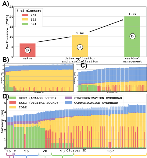
## Performance and Latency Analysis: Multi-Cluster System
### Overview
The image is a composite technical figure containing four distinct panels (A, B, C, D) that analyze the performance and latency characteristics of a computational system across different clusters and optimization strategies. Panel A is a bar chart comparing performance. Panels B and C are stacked bar charts showing latency distributions. Panel D is a detailed stacked bar chart breaking down latency components for specific clusters.
### Components/Axes
**Panel A: Performance Comparison**
* **Chart Type:** Bar Chart
* **Y-Axis:** Label: "Performance [TOPS]". Scale: 0 to 25, with major ticks at 0, 5, 10, 15, 20, 25.
* **X-Axis:** Three categorical labels: "naive", "data-replication and parallelisation", "residual management".
* **Legend:** Located in the top-left corner. Title: "# of clusters". Color-coded categories:
* Red square: 261
* Yellow square: 322
* Green square: 324
* **Data Series:** Three bars, each corresponding to an x-axis category and colored according to the legend.
* **Annotations:** Each bar contains a circled letter (B, C, D) and a performance multiplier arrow above it.
**Panels B & C: Latency Distribution**
* **Chart Type:** Stacked Bar Charts (Histogram-like)
* **Y-Axis (Both):** Label: "Latency [ms]". Scale: 0 to 3, with major ticks at 0, 1, 2, 3.
* **X-Axis (Both):** Label: "Cluster ID". The axis displays a range of cluster IDs, but specific values are not labeled on the axis ticks in these panels.
* **Data Series:** Each vertical bar represents a cluster and is stacked with colored segments representing different latency components.
**Panel D: Detailed Latency Breakdown**
* **Chart Type:** Stacked Bar Chart
* **Y-Axis:** Label: "Latency [ms]". Scale: 0 to 5, with major ticks at 0, 1, 2, 3, 4, 5.
* **X-Axis:** Label: "Cluster ID". Specific labeled ticks: 16, 2, 56, 28, 53, 167.
* **Legend:** Located in the bottom-left corner of the panel. Color-coded categories:
* Green: EXEC (ANALOG BOUND)
* Red: EXEC (DIGITAL BOUND)
* Yellow: IDLE
* Purple: SYNCHRONIZATION OVERHEAD
* Blue: COMMUNICATION OVERHEAD
* **Data Series:** Six stacked bars, one for each labeled Cluster ID on the x-axis.
### Detailed Analysis
**Panel A Analysis:**
* **Trend:** Performance increases significantly from left to right across the optimization strategies.
* **Data Points (Approximate):**
* **"naive" (Red Bar, 261 clusters):** Performance ≈ 6.5 TOPS. Annotated with circled "B".
* **"data-replication and parallelisation" (Yellow Bar, 322 clusters):** Performance ≈ 10.5 TOPS. Annotated with circled "C". An arrow from the first bar indicates a **1.6x** performance multiplier.
* **"residual management" (Green Bar, 324 clusters):** Performance ≈ 20 TOPS. Annotated with circled "D". An arrow from the second bar indicates a **1.9x** performance multiplier (relative to the second bar).
**Panel B & C Analysis:**
* These panels show the distribution of total latency across many clusters (the exact number is not specified on the axis).
* **Trend:** Latency varies considerably between clusters. The stacked composition shows that the contribution of different components (colors) to the total latency also varies.
* **Visual Comparison:** Panel B and Panel C appear to show distributions for different scenarios or configurations, but the specific titles or differentiating labels for B vs. C are not present in the image itself. The circled letters "B" and "C" in Panel A likely correspond to these charts.
**Panel D Analysis (Cluster-Specific Breakdown):**
* **Cluster 16:** Total latency ≈ 4.8 ms. Dominated by **COMMUNICATION OVERHEAD (Blue)** and **IDLE (Yellow)** time. Contains a small amount of SYNCHRONIZATION OVERHEAD (Purple).
* **Cluster 2:** Total latency ≈ 3.8 ms. Significant **IDLE (Yellow)** time, with notable EXEC (ANALOG BOUND) (Green) and EXEC (DIGITAL BOUND) (Red).
* **Cluster 56:** Total latency ≈ 3.5 ms. Similar composition to Cluster 2, with a slightly larger EXEC (DIGITAL BOUND) (Red) component.
* **Cluster 28:** Total latency ≈ 3.2 ms. Lower overall latency. Composition is mixed, with IDLE, EXEC (ANALOG), and EXEC (DIGITAL) all present.
* **Cluster 53:** Total latency ≈ 3.0 ms. Similar profile to Cluster 28.
* **Cluster 167:** Total latency ≈ 2.8 ms. The lowest total latency among the shown clusters. Composed primarily of EXEC (ANALOG BOUND) (Green) and IDLE (Yellow).
### Key Observations
1. **Performance Scaling:** The "residual management" strategy (Panel A, Green) delivers the highest performance (≈20 TOPS), nearly double that of the "data-replication" strategy and over triple that of the "naive" approach.
2. **Latency Heterogeneity:** There is significant variability in both total latency and its composition across different clusters (Panels B, C, D). This suggests non-uniform workload or hardware characteristics.
3. **Dominant Latency Components:** For the specific clusters shown in Panel D, **IDLE time (Yellow)** and **COMMUNICATION OVERHEAD (Blue)** are frequently the largest contributors to total latency, especially for higher-latency clusters like 16 and 2.
4. **Optimization Impact:** The progression from Panel A's "naive" (B) to "data-replication" (C) to "residual management" (D) correlates with the detailed latency breakdowns shown in the corresponding panels below, suggesting these are the latency profiles for those specific optimization stages.
### Interpretation
This figure demonstrates the performance benefits and latency trade-offs of different optimization techniques in a multi-cluster computing system. The "residual management" technique is clearly superior in terms of raw throughput (TOPS). However, the latency analysis reveals a complex picture: even with high performance, individual clusters experience varying delays due to different bottlenecks.
The high **IDLE** time suggests load imbalance or inefficient task scheduling, where some clusters wait for work. The significant **COMMUNICATION OVERHEAD**, particularly in Cluster 16, points to potential network congestion or inefficient data transfer protocols between clusters. The presence of both **ANALOG** and **DIGITAL** execution bounds indicates a heterogeneous processing pipeline where different stages of computation are limited by different factors (e.g., analog sensor processing vs. digital logic).
The key takeaway is that optimizing for peak performance (TOPS) does not necessarily minimize or homogenize latency. A holistic system design must address both throughput and the sources of latency variability (communication, synchronization, idle time) to ensure consistent and predictable performance across all nodes in the cluster fabric. The "residual management" approach likely improves performance by better overlapping or hiding these latency components, but their underlying causes remain visible in the per-cluster breakdown.
DECODING INTELLIGENCE...