## Hierarchical Diagram: Multi-Level Variable Structure
### Overview
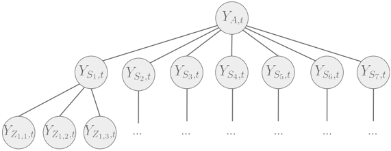
The image displays a technical hierarchical diagram, specifically a tree structure, illustrating relationships between variables indexed by time `t`. The diagram is monochromatic (black lines and text on a white background) and uses standard mathematical notation with subscripts. It represents a three-level hierarchy with a root node, first-level child nodes, and second-level child nodes (partially shown).
### Components/Axes
The diagram consists of circular nodes connected by straight lines, indicating parent-child relationships. All nodes contain mathematical variable labels.
**Node Labels (from top to bottom, left to right):**
1. **Root Node (Top Center):** `Y_{A,t}`
2. **First-Level Child Nodes (Middle Row, left to right):**
* `Y_{S_1,t}`
* `Y_{S_2,t}`
* `Y_{S_3,t}`
* `Y_{S_4,t}`
* `Y_{S_5,t}`
* `Y_{S_6,t}`
* `Y_{S_7,t}`
3. **Second-Level Child Nodes (Bottom Row, under `Y_{S_1,t}`):**
* `Y_{Z_{1,1},t}`
* `Y_{Z_{1,2},t}`
* `Y_{Z_{1,3},t}`
4. **Ellipses:** Below nodes `Y_{S_2,t}` through `Y_{S_7,t}`, vertical ellipses (`...`) are present, indicating that each of these nodes has additional, unspecified child nodes following the same pattern as `Y_{S_1,t}`.
**Spatial Grounding:**
* The root node `Y_{A,t}` is positioned at the top center.
* The seven first-level nodes are arranged in a horizontal row directly beneath the root, connected to it by lines fanning out from the root's base.
* The three second-level nodes are arranged in a horizontal row beneath `Y_{S_1,t}`, connected to it by lines fanning out from its base.
* The ellipses are centered vertically below their respective parent nodes (`Y_{S_2,t}` to `Y_{S_7,t}`).
### Detailed Analysis
The diagram defines a clear hierarchical dependency structure.
* **Level 1 (Root):** A single aggregate or top-level variable, `Y_{A,t}`.
* **Level 2 (Components):** The root variable is composed of or depends on seven sub-variables, `Y_{S_1,t}` through `Y_{S_7,t}`. The subscript `S` likely denotes a "Sector," "Segment," or "Source."
* **Level 3 (Sub-Components):** Each Level 2 variable is further decomposed. The diagram explicitly shows the decomposition for `Y_{S_1,t}` into three sub-variables: `Y_{Z_{1,1},t}`, `Y_{Z_{1,2},t}`, and `Y_{Z_{1,3},t}`. The subscript `Z` with double indices (e.g., `Z_{1,1}`) suggests a finer granularity, such as "Zone," "Item," or "Sub-source" within the first sector (`S_1`).
* **Temporal Index:** Every variable includes the subscript `t`, indicating that this entire structure is time-indexed. This implies the diagram represents a snapshot of a dynamic system at time `t`, or that the relationships are defined for each time period.
* **Symmetry and Pattern:** The consistent use of ellipses under `Y_{S_2,t}` to `Y_{S_7,t}` strongly implies a symmetric structure. It is inferred that each of these six nodes also has multiple child nodes (likely three, following the pattern of `Y_{S_1,t}`), but they are not drawn to avoid clutter.
### Key Observations
1. **Strict Hierarchy:** The structure is a strict tree with no cross-connections or cycles. Each node (except the root) has exactly one parent.
2. **Consistent Notation:** The variable naming follows a strict pattern: `Y` is the base variable, the first subscript denotes the level/component (`A`, `S_i`, `Z_{i,j}`), and the final subscript `t` denotes time.
3. **Scalability:** The diagram is designed to represent a potentially large system. Showing only the full decomposition for the first branch (`S_1`) while using ellipses for others is a common technical illustration technique to convey pattern without visual overload.
4. **Abstraction:** The diagram is abstract. It does not specify what `Y`, `A`, `S`, or `Z` represent (e.g., sales, sensor readings, financial metrics), making it a general template for hierarchical modeling.
### Interpretation
This diagram is a formal representation of a **hierarchical decomposition model**. It is commonly used in fields like econometrics, statistics, machine learning, and systems engineering.
* **What it Suggests:** The data or system being modeled has a natural nested structure. The top-level aggregate `Y_{A,t}` (e.g., total national sales) is the sum or function of several mid-level components `Y_{S_i,t}` (e.g., sales in seven regions), each of which is itself composed of multiple low-level elements `Y_{Z_{i,j},t}` (e.g., sales in individual stores within a region).
* **Relationships:** The lines represent a "consists-of" or "is driven-by" relationship. The value of a parent node at time `t` is determined by the values of its child nodes at the same time `t`. This is foundational for **hierarchical time series forecasting**, where forecasts are generated at multiple levels of aggregation and must be coherent (i.e., sum up correctly).
* **Notable Pattern:** The explicit showing of three children for `S_1` and the implied symmetry for `S_2`-`S_7` suggests a balanced hierarchy at the second level, though the number of children per node could vary in practice. The use of `t` on all nodes is critical—it frames this as a dynamic, time-varying system rather than a static taxonomy.
* **Underlying Purpose:** This structure enables analysis at different scales. One can analyze the behavior of the whole system (`A`), individual sectors (`S_i`), or granular units (`Z_{i,j}`). It also facilitates information flow, where data from the bottom level propagates up to inform the state of the higher levels.