\n
## 3D Scatter Plot: Latent vs. Vocabulary Token Distribution
### Overview
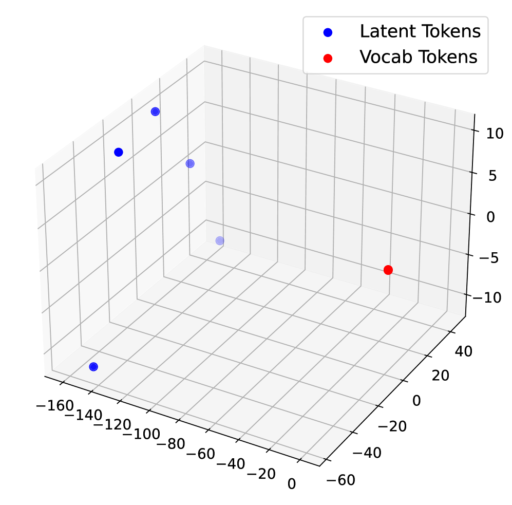
This image is a 3D scatter plot visualizing the spatial distribution of two distinct categories of tokens within a three-dimensional embedding space. The plot compares "Latent Tokens" (represented by blue spheres) and "Vocab Tokens" (represented by a single red sphere). The visualization suggests an analysis of how different token types are positioned relative to each other in a learned vector space.
### Components/Axes
* **Chart Type:** 3D Scatter Plot.
* **Legend:** Located in the top-right corner of the plot area.
* **Blue Circle:** Labeled "Latent Tokens".
* **Red Circle:** Labeled "Vocab Tokens".
* **Axes:** The plot has three orthogonal axes forming a 3D grid. The axes are not explicitly labeled with names (e.g., "Dimension 1", "PC1"), but their numerical scales are visible.
* **X-Axis (Front-Left to Back-Right):** Scale ranges from approximately -160 to 0. Major tick marks are at intervals of 20 (-160, -140, -120, -100, -80, -60, -40, -20, 0).
* **Y-Axis (Front-Right to Back-Left):** Scale ranges from approximately -60 to 40. Major tick marks are at intervals of 20 (-60, -40, -20, 0, 20, 40).
* **Z-Axis (Vertical):** Scale ranges from approximately -10 to 10. Major tick marks are at intervals of 5 (-10, -5, 0, 5, 10).
* **Grid:** A light gray grid is present on the three back planes of the 3D cube to aid in spatial orientation.
### Detailed Analysis
**Data Points and Approximate Coordinates:**
The plot contains a total of 7 visible data points. Coordinates are estimated based on their position relative to the grid lines and axis ticks.
1. **Latent Tokens (Blue Spheres):** There are 6 blue points scattered throughout the space.
* **Point B1 (Top-Left Cluster):** Positioned high on the Z-axis. Approximate coordinates: (X: -140, Y: 20, Z: 8).
* **Point B2 (Top-Left Cluster):** Near B1. Approximate coordinates: (X: -120, Y: 10, Z: 6).
* **Point B3 (Top-Left Cluster):** Near B1 and B2. Approximate coordinates: (X: -100, Y: 0, Z: 4).
* **Point B4 (Center-Left):** Lower and more central than the top-left cluster. Approximate coordinates: (X: -80, Y: -10, Z: -2).
* **Point B5 (Bottom-Left):** The lowest point on the Z-axis and far left on the X-axis. Approximate coordinates: (X: -150, Y: -50, Z: -8).
* **Point B6 (Center, Faint):** Appears slightly faded, possibly indicating depth or a different property. Approximate coordinates: (X: -60, Y: -20, Z: -4).
2. **Vocab Tokens (Red Sphere):** There is 1 red point.
* **Point R1:** Positioned in the right half of the space, isolated from the blue points. Approximate coordinates: (X: -20, Y: 30, Z: -6).
**Visual Trend Verification:**
* **Latent Tokens (Blue):** The series does not form a single linear trend. Instead, it shows a scattered distribution with a loose cluster in the upper-left quadrant (high Z, negative X and Y) and a few outlying points, including one at the extreme bottom-left.
* **Vocab Token (Red):** As a single point, it has no trend. Its key characteristic is its spatial separation from the cluster of blue points.
### Key Observations
1. **Spatial Separation:** The single "Vocab Token" (red) is located in a distinct region of the 3D space (positive Y, less negative X) compared to the majority of the "Latent Tokens" (blue), which are concentrated in areas with more negative X and Y values.
2. **Clustering vs. Isolation:** The "Latent Tokens" exhibit some clustering, particularly three points in the top-left region. In contrast, the "Vocab Token" is isolated.
3. **Range of Distribution:** The "Latent Tokens" span a wide range across all three dimensions, especially on the X-axis (from ~-150 to -60) and Z-axis (from ~-8 to +8). The "Vocab Token" occupies a more specific, mid-range location.
4. **Point Fading:** One blue point (B6) appears slightly more transparent or faded than the others, which could be a rendering artifact to show depth or might indicate a different sub-category or property.
### Interpretation
This plot likely visualizes the output of a dimensionality reduction technique (like PCA or t-SNE) applied to token embeddings from a language or machine learning model. The clear spatial separation between the red "Vocab Token" and the blue "Latent Tokens" suggests these two categories occupy fundamentally different regions in the model's embedding space.
* **What it suggests:** "Vocab Tokens" may represent standard, discrete tokens from the model's fixed vocabulary (e.g., words or subwords). "Latent Tokens" could represent continuous, learned vectors from an intermediate layer of the model, which encode more abstract or contextual information. Their scattered distribution might reflect the diverse semantic or syntactic roles these latent representations capture.
* **Why it matters:** The separation indicates that the model's internal, latent representations are not simply a direct mapping of its input vocabulary tokens. They form a distinct, possibly more nuanced, subspace. Analyzing this geometry can provide insights into how the model organizes information, how concepts are related internally, and could be used for tasks like probing model understanding or detecting anomalies.
* **Notable Anomaly:** The presence of a single "Vocab Token" is unusual. Typically, one would expect many vocabulary tokens to be plotted. This could be a specific example chosen for comparison, an average point, or a token of particular interest. Its isolation highlights the distinct nature of the latent space.