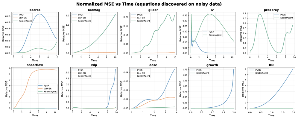
\n ## Line Charts: Normalized MSE vs Time (equations discovered on noisy data) ### Overview The image presents a series of ten line charts, each depicting the relationship between Normalized Mean Squared Error (MSE) and Time. Each chart represents a different equation discovery scenario (bacres, barmag, glider, lv, predprey, shearflow, vdp, dosc, growth, RD). Three different methods – PySR, LLM-SR, and KeplerAgent – are compared within each chart, indicated by different colored lines. The charts aim to visualize how well each method converges to a solution (lower MSE) over time. ### Components/Axes * **X-axis:** Time, ranging from 0 to 10 (except for 'dosc' which ranges to 3, 'growth' which ranges to 2.5, and 'RD' which ranges to 2.0). * **Y-axis:** Relative MSE, with varying scales for each chart. * **Legend:** Located in the top-left corner of each chart, identifying the lines as: * PySR (represented by a dark turquoise line) * LLM-SR (represented by an orange line) * KeplerAgent (represented by a teal line) * **Chart Titles:** Each chart is labeled with the name of the equation discovery scenario (e.g., "bacres", "barmag"). * **Overall Title:** "Normalized MSE vs Time (equations discovered on noisy data)" positioned at the top center of the image. ### Detailed Analysis or Content Details Here's a breakdown of each chart, including observed trends and approximate data points. Note that values are estimated from the visual representation. 1. **bacres:** * PySR: Line starts at approximately 0.02, increases to around 0.04 at time 2, then decreases to approximately 0.01 by time 10. * LLM-SR: Line starts at approximately 0.03, increases to around 0.05 at time 2, then decreases to approximately 0.02 by time 10. * KeplerAgent: Line starts at approximately 0.03, remains relatively flat around 0.03-0.04 until time 6, then decreases to approximately 0.01 by time 10. 2. **barmag:** * PySR: Line slopes upward, starting at approximately 0.1 at time 0, reaching around 1.8 at time 10. * LLM-SR: Line slopes upward, starting at approximately 0.1 at time 0, reaching around 1.9 at time 10. * KeplerAgent: Line slopes downward, starting at approximately 0.2 at time 0, reaching around 0.05 at time 10. 3. **glider:** * PySR: Line slopes downward, starting at approximately 0.15 at time 0, reaching around 0.01 at time 10. * LLM-SR: Line slopes downward, starting at approximately 0.15 at time 0, reaching around 0.02 at time 10. * KeplerAgent: Line slopes downward, starting at approximately 0.15 at time 0, reaching around 0.01 at time 10. 4. **lv:** * PySR: Line slopes downward, starting at approximately 0.3 at time 0, reaching around 0.05 at time 10. * KeplerAgent: Line slopes downward, starting at approximately 0.3 at time 0, reaching around 0.03 at time 10. 5. **predprey:** * PySR: Line fluctuates, starting at approximately 0.7 at time 0, reaching around 0.6 at time 10. * LLM-SR: Line fluctuates, starting at approximately 0.7 at time 0, reaching around 0.6 at time 10. * KeplerAgent: Line fluctuates, starting at approximately 0.7 at time 0, reaching around 0.5 at time 10. 6. **shearflow:** * PySR: Line slopes downward rapidly, starting at approximately 0.05 at time 0, reaching around 0.001 at time 10. * LLM-SR: Line slopes downward rapidly, starting at approximately 0.05 at time 0, reaching around 0.001 at time 10. * KeplerAgent: Line slopes downward rapidly, starting at approximately 0.05 at time 0, reaching around 0.001 at time 10. 7. **vdp:** * PySR: Line fluctuates, starting at approximately 15 at time 0, reaching around 1.5 at time 10. * LLM-SR: Line fluctuates, starting at approximately 15 at time 0, reaching around 2 at time 10. * KeplerAgent: Line slopes downward, starting at approximately 15 at time 0, reaching around 0.5 at time 10. 8. **dosc:** * PySR: Line slopes downward, starting at approximately 0.04 at time 0, reaching around 0.005 at time 3. * LLM-SR: Line slopes downward, starting at approximately 0.04 at time 0, reaching around 0.01 at time 3. * KeplerAgent: Line slopes downward, starting at approximately 0.04 at time 0, reaching around 0.005 at time 3. 9. **growth:** * PySR: Line slopes downward, starting at approximately 1.75 at time 0, reaching around 0.2 at time 2.5. * LLM-SR: Line slopes downward, starting at approximately 1.75 at time 0, reaching around 0.3 at time 2.5. * KeplerAgent: Line slopes downward, starting at approximately 1.75 at time 0, reaching around 0.2 at time 2.5. 10. **RD:** * PySR: Line slopes downward, starting at approximately 6 at time 0, reaching around 0.5 at time 2. * LLM-SR: Line slopes downward, starting at approximately 6 at time 0, reaching around 1 at time 2. * KeplerAgent: Line slopes downward, starting at approximately 6 at time 0, reaching around 0.5 at time 2. ### Key Observations * PySR and KeplerAgent often exhibit similar downward trends, indicating faster convergence to lower MSE values in many scenarios. * LLM-SR often shows a slower convergence rate or higher final MSE values compared to PySR and KeplerAgent. * The 'barmag' chart is an outlier, where both PySR and LLM-SR show increasing MSE over time, while KeplerAgent decreases. * The 'predprey' and 'vdp' charts show fluctuating MSE values for all three methods, suggesting instability in the equation discovery process for these scenarios. * The scale of the Y-axis (Relative MSE) varies significantly between charts, making direct comparison of MSE values across different scenarios difficult. ### Interpretation The charts demonstrate the performance of three different equation discovery methods (PySR, LLM-SR, and KeplerAgent) on a variety of equations with noisy data. Generally, PySR and KeplerAgent appear to be more effective at finding solutions (reducing MSE) than LLM-SR. The 'barmag' scenario is a notable exception, suggesting that KeplerAgent may be more robust to certain types of noise or equation structures. The fluctuating MSE values in 'predprey' and 'vdp' indicate that these equations may be particularly challenging to discover, potentially due to high complexity or sensitivity to initial conditions. The varying Y-axis scales highlight the importance of considering the specific context of each equation when interpreting the results. The overall trend suggests that symbolic regression techniques (PySR and KeplerAgent) are more reliable for equation discovery in this setting, while LLM-SR may require further refinement or be better suited for different types of problems.