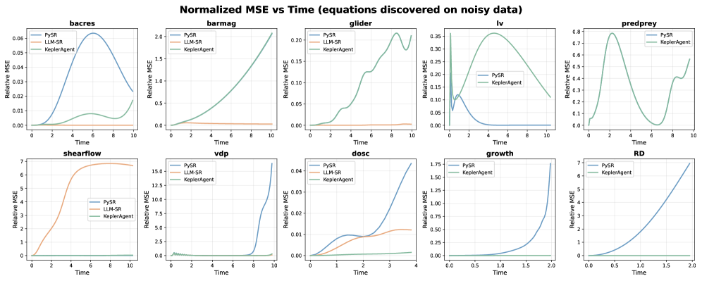
## Line Graphs: Normalized MSE vs Time (equations discovered on noisy data)
### Overview
The image displays 10 line graphs arranged in a 2x5 grid, comparing the performance of three methods (PySR, LLM-SR, KeplerAgent) across different datasets. Each graph plots **Relative MSE** against **Time**, with datasets labeled as: `bacres`, `barmag`, `glider`, `iv`, `predprey`, `shearflow`, `vdp`, `dosc`, `growth`, and `RD`. The y-axis scales vary per subplot, while the x-axis consistently ranges from 0 to 10 (or shorter for `growth` and `RD`).
---
### Components/Axes
- **Main Title**: "Normalized MSE vs Time (equations discovered on noisy data)" (centered at top).
- **Subplot Titles**: Dataset names (e.g., `bacres`, `barmag`) positioned above each graph.
- **X-Axis**: Labeled "Time" (horizontal), with ticks at 0, 2, 4, 6, 8, 10 (or shorter for `growth`/`RD`).
- **Y-Axis**: Labeled "Relative MSE" (vertical), with scales varying per subplot (e.g., 0–0.06 for `bacres`, 0–7 for `shearflow`).
- **Legend**: Top-right corner of each subplot, with:
- **Blue**: PySR
- **Orange**: LLM-SR
- **Green**: KeplerAgent
---
### Detailed Analysis
#### bacres
- **PySR (blue)**: Peaks at ~0.06 MSE around time 5, then declines.
- **LLM-SR (orange)**: Flat line near 0.005 MSE.
- **KeplerAgent (green)**: Gradual increase from 0.005 to 0.015 MSE.
#### barmag
- **PySR (blue)**: Flat near 0.005 MSE.
- **LLM-SR (orange)**: Flat near 0.005 MSE.
- **KeplerAgent (green)**: Steady rise from 0.005 to 2.0 MSE.
#### glider
- **PySR (blue)**: Flat near 0.005 MSE.
- **LLM-SR (orange)**: Flat near 0.005 MSE.
- **KeplerAgent (green)**: Sharp rise from 0.005 to 0.2 MSE by time 10.
#### iv
- **PySR (blue)**: Sharp peak at ~0.1 MSE at time 1, then drops to 0.005.
- **KeplerAgent (green)**: Peaks at ~0.35 MSE at time 3, then declines to 0.15.
#### predprey
- **PySR (blue)**: Flat near 0.005 MSE.
- **KeplerAgent (green)**: Peaks at ~0.75 MSE at time 2, then oscillates between 0.1 and 0.6.
#### shearflow
- **LLM-SR (orange)**: Sharp rise from 0 to 7 MSE by time 6, then plateaus.
- **KeplerAgent (green)**: Flat near 0.005 MSE.
#### vdp
- **PySR (blue)**: Flat near 0.005 MSE until time 8, then spikes to 15 MSE.
- **KeplerAgent (green)**: Flat near 0.005 MSE.
#### dosc
- **PySR (blue)**: Gradual rise from 0.005 to 0.04 MSE by time 4.
- **LLM-SR (orange)**: Gradual rise from 0.005 to 0.015 MSE by time 4.
- **KeplerAgent (green)**: Flat near 0.005 MSE.
#### growth
- **PySR (blue)**: Sharp rise from 0 to 1.75 MSE by time 2.
- **KeplerAgent (green)**: Flat near 0.005 MSE.
#### RD
- **PySR (blue)**: Gradual rise from 0 to 7 MSE by time 2.
- **KeplerAgent (green)**: Flat near 0.005 MSE.
---
### Key Observations
1. **KeplerAgent Dominance**: Outperforms other methods in most datasets (e.g., `bacres`, `barmag`, `predprey`), maintaining lower MSE.
2. **PySR Limitations**: Struggles with noisy data in `vdp` (spike at time 10) and `RD` (steady rise).
3. **LLM-SR Variability**: Performs well in `shearflow` (low MSE) but is absent in `glider`, `iv`, and `vdp`.
4. **Time Sensitivity**: Methods like PySR and KeplerAgent show time-dependent performance (e.g., `bacres` peak at time 5, `growth` spike at time 2).
5. **Missing Data**: LLM-SR is absent in `glider`, `iv`, and `vdp` subplots.
---
### Interpretation
The data suggests **KeplerAgent** is robust to noisy data across most datasets, consistently achieving lower MSE. **PySR** exhibits instability in certain scenarios (e.g., `vdp`, `RD`), while **LLM-SR** shows promise in `shearflow` but lacks broader applicability. The absence of LLM-SR in some subplots may indicate method-specific limitations or data incompatibility. Timeframes vary per dataset, implying differing problem complexities. Overall, KeplerAgent’s performance highlights its potential for real-world applications requiring noise resilience.