## Line Graph: Effective Dimension Scaling
### Overview
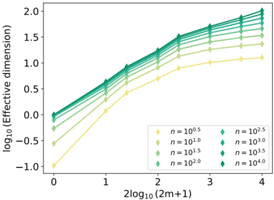
The image is a line graph plotting the base-10 logarithm of an "Effective dimension" against a transformed parameter "2log₁₀(2m+1)". It displays multiple data series, each corresponding to a different value of a parameter `n`, showing how the effective dimension scales with the x-axis variable for different `n`.
### Components/Axes
* **Chart Type:** Multi-line graph with markers.
* **X-Axis:**
* **Label:** `2log₁₀(2m+1)`
* **Scale:** Linear scale from 0 to 4, with major tick marks at 0, 1, 2, 3, and 4.
* **Y-Axis:**
* **Label:** `log₁₀(Effective dimension)`
* **Scale:** Linear scale from -1.0 to 2.0, with major tick marks at -1.0, -0.5, 0.0, 0.5, 1.0, 1.5, and 2.0.
* **Legend:**
* **Position:** Bottom-right corner of the plot area.
* **Content:** A list of 8 data series, each identified by a colored diamond marker and a label for the parameter `n`.
* **Series Labels (from top to bottom in legend):**
1. `n = 10⁰·⁵` (Light yellow-green)
2. `n = 10¹·⁰` (Light green)
3. `n = 10¹·⁵` (Medium green)
4. `n = 10²·⁰` (Green)
5. `n = 10²·⁵` (Teal green)
6. `n = 10³·⁰` (Darker teal)
7. `n = 10³·⁵` (Dark teal)
8. `n = 10⁴·⁰` (Darkest teal/blue-green)
### Detailed Analysis
Each data series is represented by a line connecting diamond-shaped markers at integer x-values (0, 1, 2, 3, 4). The lines are ordered from bottom to top in the graph, corresponding to increasing values of `n` in the legend.
**Trend Verification:** All eight lines exhibit a consistent, monotonically increasing trend. They slope upward from left to right, indicating a positive correlation between the x-axis variable and the log of the effective dimension. The slope is steepest for the lowest `n` values and becomes progressively shallower for higher `n` values.
**Data Point Extraction (Approximate Y-values for each X):**
The following table reconstructs the approximate `log₁₀(Effective dimension)` values for each series at the given `2log₁₀(2m+1)` points. Values are estimated from the graph's grid.
| `n` (Legend) | Color (Approx.) | X=0 | X=1 | X=2 | X=3 | X=4 |
| :--- | :--- | :--- | :--- | :--- | :--- | :--- |
| `10⁰·⁵` | Light yellow-green | -1.0 | 0.1 | 0.7 | 1.0 | 1.1 |
| `10¹·⁰` | Light green | -0.6 | 0.3 | 0.9 | 1.2 | 1.3 |
| `10¹·⁵` | Medium green | -0.3 | 0.5 | 1.1 | 1.4 | 1.5 |
| `10²·⁰` | Green | 0.0 | 0.6 | 1.2 | 1.5 | 1.6 |
| `10²·⁵` | Teal green | 0.0 | 0.65 | 1.25 | 1.6 | 1.7 |
| `10³·⁰` | Darker teal | 0.0 | 0.7 | 1.3 | 1.7 | 1.8 |
| `10³·⁵` | Dark teal | 0.0 | 0.7 | 1.35 | 1.75 | 1.9 |
| `10⁴·⁰` | Darkest teal | 0.0 | 0.7 | 1.4 | 1.8 | 2.0 |
**Note on X=0:** For `n >= 10²·⁰`, the lines converge at approximately `log₁₀(Effective dimension) = 0.0` when `X=0`.
### Key Observations
1. **Convergence at Low X:** For higher values of `n` (≥ 10²·⁰), the effective dimension starts at the same point (log value ~0) when the x-axis variable is 0.
2. **Divergence with Increasing X:** As the x-axis variable increases, the lines fan out. The vertical separation between lines for different `n` values becomes more pronounced.
3. **Diminishing Returns of n:** The incremental increase in the effective dimension for each tenfold increase in `n` (e.g., from 10²·⁰ to 10³·⁰) appears to decrease as `n` gets larger. The gap between the `n=10³·⁵` and `n=10⁴·⁰` lines is smaller than the gap between `n=10⁰·⁵` and `n=10¹·⁰`.
4. **Shape of Curves:** The curves are concave down, suggesting a sub-linear or logarithmic growth relationship between the effective dimension and the x-axis variable, even on this log-log-like plot.
### Interpretation
This graph demonstrates a scaling law. The "Effective dimension" of some system or model increases with the parameter `2log₁₀(2m+1)` (which likely relates to a model size or complexity parameter `m`), but the rate of increase is modulated by another parameter `n`.
* **Core Relationship:** The positive slope confirms that increasing `m` (via the x-axis) leads to a higher effective dimension, which often correlates with model capacity or representational power.
* **Role of `n`:** The parameter `n` acts as a scaling factor. A larger `n` results in a higher effective dimension for the same `m`. However, the effect of increasing `n` shows diminishing returns, as seen by the converging lines at the top of the graph.
* **Practical Implication:** In a machine learning context, this could illustrate that both model width (`n`) and depth/complexity (`m`) contribute to effective capacity, but there is an optimal balance. Simply increasing one parameter indefinitely yields progressively smaller gains. The convergence at `X=0` for high `n` might indicate a baseline capacity threshold.
* **Underlying Model:** The specific functional form `2log₁₀(2m+1)` suggests the relationship involves a logarithmic transformation of a term linear in `m`. The graph's concave shape implies the effective dimension grows slower than exponentially with `m`, possibly following a power law.