## System Architecture Diagram: Signal Processing and Control Flow
### Overview
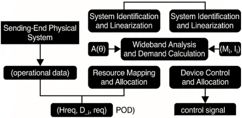
The image displays a technical flowchart or system architecture diagram illustrating a multi-stage process for transforming operational data from a physical system into control signals. The diagram uses black rectangular boxes with white text to represent processing stages or components, connected by black arrows indicating the direction of data or signal flow. The overall flow moves generally from left to right, with some parallel processing paths.
### Components/Axes
The diagram is composed of the following labeled components, listed in approximate spatial order from left to right and top to bottom:
1. **Sending-End Physical System** (Top-left)
2. **(operational data)** (Below component 1)
3. **System Identification and Linearization** (Top-center)
4. **System Identification and Linearization** (Top-right, duplicate of component 3)
5. **A(θ)** (Small box, left of center)
6. **Wideband Analysis and Demand Calculation** (Center)
7. **(M_i, I_i)** (Small box, right of center)
8. **Resource Mapping and Allocation** (Below component 6)
9. **Device Control and Allocation** (Bottom-right)
10. **(Hreq, D_i, req)** (Bottom-center, left of component 11)
11. **POD** (Bottom-center, right of component 10)
12. **control signal** (Bottom-right, below component 9)
### Detailed Analysis
**Flow and Connections:**
* The process originates from the **Sending-End Physical System**.
* An arrow points downward from this system to **(operational data)**, indicating data extraction.
* From **(operational data)**, a line flows rightward and splits. One branch goes up to **System Identification and Linearization** (top-center). The other continues right to **Resource Mapping and Allocation**.
* The two **System Identification and Linearization** blocks (top-center and top-right) appear to be parallel or redundant processes. They both feed into the central **Wideband Analysis and Demand Calculation** block.
* The input **A(θ)** feeds into the left side of the **Wideband Analysis and Demand Calculation** block.
* The input **(M_i, I_i)** feeds into the right side of the **Wideband Analysis and Demand Calculation** block.
* The output of **Wideband Analysis and Demand Calculation** flows downward to **Resource Mapping and Allocation**.
* The output of **Resource Mapping and Allocation** flows rightward to **Device Control and Allocation**.
* The output of **Device Control and Allocation** flows downward to produce the final **control signal**.
* A separate data tuple **(Hreq, D_i, req)** and the label **POD** are positioned at the bottom, connected by a line that appears to feed into the **Resource Mapping and Allocation** block from below.
**Text Transcription:**
All text is in English. The precise transcription of labels and mathematical notations is as follows:
* Sending-End Physical System
* (operational data)
* System Identification and Linearization
* A(θ)
* Wideband Analysis and Demand Calculation
* (M_i, I_i)
* Resource Mapping and Allocation
* Device Control and Allocation
* (Hreq, D_i, req)
* POD
* control signal
### Key Observations
1. **Duplicate Component:** The label "System Identification and Linearization" appears twice in identical boxes at the top of the diagram. This suggests either a parallel processing step for different subsystems or a visual representation of a repeated process.
2. **Mathematical Inputs:** The central processing block (**Wideband Analysis and Demand Calculation**) receives two specific mathematical inputs: **A(θ)** (likely a parameterized matrix or function) and **(M_i, I_i)** (likely a tuple representing mass/inertia or other physical parameters for component *i*).
3. **Data Tuple at Base:** The tuple **(Hreq, D_i, req)** and the acronym **POD** are positioned at the bottom, feeding into the resource allocation stage. This likely represents requirement specifications (e.g., *Hreq* for a requirement, *D_i* for a device parameter, *req* for a request) and a method or data type (POD could stand for "Plain Old Data" or a domain-specific acronym).
4. **Linear Flow with Parallel Start:** The core process is linear (Data -> Analysis -> Resource Mapping -> Device Control -> Signal), but it begins with parallel paths for system identification and incorporates multiple external parameter inputs.
### Interpretation
This diagram models a **cyber-physical control system**, likely for a complex engineering application such as robotics, aerospace, or industrial automation. The process begins with the physical world ("Sending-End Physical System") and ends with a digital "control signal" meant to actuate that system.
The flow demonstrates a classic sense-think-act cycle:
1. **Sense:** Operational data is collected from the physical system.
2. **Think/Process:** This data undergoes sophisticated analysis. "System Identification and Linearization" suggests creating a mathematical model of the physical system's behavior. "Wideband Analysis and Demand Calculation" implies evaluating system performance across a range of frequencies or conditions to determine operational demands. "Resource Mapping and Allocation" then plans how to meet those demands using available computational or physical resources.
3. **Act:** "Device Control and Allocation" translates the resource plan into specific commands, resulting in the final "control signal."
The presence of parameters like **A(θ)** and **(M_i, I_i)** indicates the system's decisions are model-based, relying on mathematical representations of the system's dynamics and physical properties. The input **(Hreq, D_i, req)** suggests the process is also driven by external requirements or constraints.
**Notable Anomaly:** The duplicate "System Identification and Linearization" block is the most striking feature. It could indicate that two separate subsystems are being modeled in parallel, or it might be a diagrammatic error. Without additional context, its exact purpose is ambiguous, but it highlights that system modeling is a critical, possibly multi-faceted, initial step in this pipeline.