# Technical Data Extraction: MPC Performance Comparison
This document provides a detailed technical extraction of the data and trends presented in the provided image, which consists of two side-by-side plots comparing "Optimal MPC" and "TD-MPC" (Temporal Difference Model Predictive Control).
---
## 1. Left Plot: Phase Portrait (State Space Trajectory)
### Component Isolation:
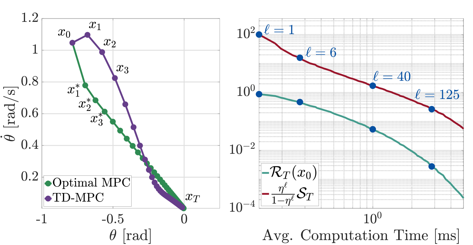
- **Type:** 2D Line Plot with markers.
- **Y-Axis:** $\dot{\theta}$ [rad/s] (Angular Velocity). Scale: 0 to 1.2.
- **X-Axis:** $\theta$ [rad] (Angle). Scale: -1 to 0.
- **Legend Location:** Bottom-left [x $\approx$ 0.1, y $\approx$ 0.1].
### Legend and Data Series:
1. **Optimal MPC (Green Line/Markers):**
* **Trend:** Slopes downward and to the right in a relatively direct, smooth curve toward the origin (0,0).
* **Key Points:**
* Starts at $x_0$ (shared with TD-MPC).
* Labeled intermediate points: $x_1^*$, $x_2^*$, $x_3^*$.
* Ends at $x_T$ (0, 0).
2. **TD-MPC (Purple Line/Markers):**
* **Trend:** Initially moves upward and slightly right (increasing $\dot{\theta}$), then curves sharply downward and right. It follows a wider arc than the Optimal MPC before converging to the same terminal point.
* **Key Points:**
* Starts at $x_0 \approx (-0.8, 1.05)$.
* Labeled intermediate points: $x_1$, $x_2$, $x_3$.
* Ends at $x_T$ (0, 0).
### Spatial Grounding & Observations:
- The TD-MPC trajectory ($x_1, x_2, x_3$) deviates significantly from the Optimal MPC trajectory ($x_1^*, x_2^*, x_3^*$) in the early stages of the movement.
- Both trajectories converge at the terminal state $x_T$ at the origin.
---
## 2. Right Plot: Computational Efficiency vs. Regret
### Component Isolation:
- **Type:** Log-Log Scale Line Plot.
- **Y-Axis:** Logarithmic scale from $10^{-4}$ to $10^2$.
- **X-Axis:** Avg. Computation Time [ms]. Logarithmic scale from approx. $10^{-1}$ to $10^1$.
- **Legend Location:** Bottom-left [x $\approx$ 0.55, y $\approx$ 0.2].
### Legend and Data Series:
1. **$\mathcal{R}_T(x_0)$ (Teal/Cyan Line):**
* **Trend:** Slopes downward (negative correlation). As computation time increases, the value of $\mathcal{R}_T(x_0)$ decreases significantly.
* **Visual Check:** The line is positioned below the red dashed line.
2. **$\frac{\eta^\ell}{1-\eta^\ell} \mathcal{S}_T$ (Dark Red Dashed Line):**
* **Trend:** Slopes downward. This represents a theoretical upper bound or a related metric that also improves with more computation time.
* **Visual Check:** This line maintains a higher value than the teal line across the entire x-axis range.
### Annotated Data Points (Blue Circles):
The plot identifies specific points on both lines corresponding to different values of $\ell$ (likely iterations or look-ahead depth):
* **$\ell = 1$:** Located at the far left (lowest computation time, highest error/regret).
* **$\ell = 6$:** Located at approx. $3 \times 10^{-1}$ ms.
* **$\ell = 40$:** Located at $10^0$ (1 ms).
* **$\ell = 125$:** Located at approx. $4 \times 10^0$ ms.
### Trend Verification:
- There is a clear power-law relationship (linear on a log-log scale) between computation time and the performance metrics.
- Increasing the parameter $\ell$ increases computation time but results in a logarithmic decrease in the regret/error metrics.
---
## 3. Textual Transcriptions
### Mathematical Notations & Labels:
- **Left Plot Labels:** $x_0, x_1, x_2, x_3, x_1^*, x_2^*, x_3^*, x_T$
- **Right Plot Labels:** $\ell = 1, \ell = 6, \ell = 40, \ell = 125$
- **Legend Formulas:**
- $\mathcal{R}_T(x_0)$
- $\frac{\eta^\ell}{1-\eta^\ell} \mathcal{S}_T$
### Axis Titles:
- **Left Y:** $\dot{\theta}$ [rad/s]
- **Left X:** $\theta$ [rad]
- **Right X:** Avg. Computation Time [ms]
### Legend Text:
- Optimal MPC
- TD-MPC