## Line Chart: Execution Time vs. Max Region Size
### Overview
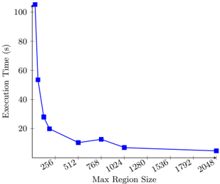
The image is a 2D line chart plotting "Execution Time" in seconds against "Max Region Size." It displays a single data series showing a clear inverse relationship: as the maximum region size increases, the execution time decreases, with the rate of decrease slowing significantly after a certain point.
### Components/Axes
* **Chart Type:** Line chart with square data point markers.
* **X-Axis (Horizontal):**
* **Label:** `Max Region Size`
* **Scale:** Linear scale.
* **Tick Marks/Values:** 256, 512, 768, 1024, 1280, 1536, 1792, 2048.
* **Y-Axis (Vertical):**
* **Label:** `Execution Time (s)`
* **Scale:** Linear scale.
* **Range:** 0 to 100+ seconds.
* **Tick Marks/Values:** 0, 20, 40, 60, 80, 100.
* **Data Series:**
* **Visual Representation:** A solid blue line connecting blue square markers.
* **Legend:** Not present, as there is only one data series.
* **Grid:** Light gray grid lines are present for both axes.
### Detailed Analysis
**Data Point Extraction (Approximate Values):**
The following table reconstructs the data based on visual alignment of the blue square markers with the axes.
| Max Region Size | Execution Time (s) |
| :-------------- | :----------------- |
| 256 | ~105 |
| 512 | ~55 |
| 768 | ~28 |
| 1024 | ~20 |
| 1280 | ~12 |
| 1536 | ~11 |
| 1792 | ~10 |
| 2048 | ~9 |
**Trend Verification:**
The blue line exhibits a steep, downward slope from left to right initially, which then flattens into a near-horizontal plateau.
1. **Steep Descent (256 to 1024):** The line drops sharply from ~105s to ~20s. The most dramatic decrease occurs between region sizes 256 and 512.
2. **Transition & Plateau (1024 to 2048):** The slope becomes much shallower. From 1024 to 1280, there is a moderate decrease from ~20s to ~12s. From 1280 onward to 2048, the line is nearly flat, showing only a very slight decrease from ~12s to ~9s.
### Key Observations
1. **Non-Linear Improvement:** The performance benefit (reduction in execution time) from increasing the Max Region Size is not linear. The greatest gains are achieved with initial increases from a small base size.
2. **Diminishing Returns:** After a Max Region Size of approximately 1024-1280, further increases yield progressively smaller reductions in execution time, indicating a point of diminishing returns.
3. **Performance Floor:** The execution time appears to approach a lower bound or "floor" of approximately 9-12 seconds for region sizes of 1280 and above.
### Interpretation
This chart demonstrates a classic performance optimization curve. The "Max Region Size" likely represents a configurable parameter for a computational task (e.g., image processing, data chunking, or parallel processing). The data suggests:
* **Optimal Range:** There is a clear "knee" in the curve around a region size of 1024-1280. Configuring the system within this range provides a strong balance between performance and resource usage (as larger regions may consume more memory).
* **System Bottleneck Shift:** The plateau indicates that beyond a certain region size, the execution time is no longer constrained by the region size itself. The limiting factor shifts to another component of the system (e.g., CPU speed, memory bandwidth, or I/O operations), which sets the observed performance floor of ~9-12 seconds.
* **Practical Guidance:** For this specific workload, setting the Max Region Size to 1280 or 1536 would be a prudent choice. It captures nearly all the performance benefit without unnecessarily allocating resources for larger sizes (1792, 2048) that provide negligible additional speedup. The chart provides empirical evidence to justify this configuration choice.