## Oscillator Sampling and Cut Analysis
### Overview
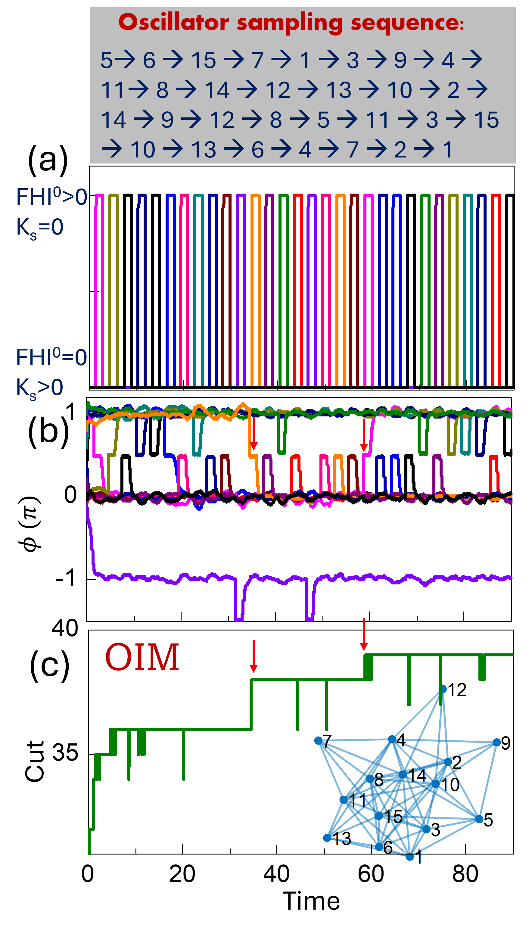
The image presents three subplots (a, b, and c) illustrating the behavior of oscillators and a related cut analysis over time. Subplot (a) shows the oscillator sampling sequence when FHI° > 0 and Ks = 0. Subplot (b) shows the phase (phi) of the oscillators when FHI° = 0 and Ks > 0. Subplot (c) shows the cut value over time, along with a network graph representing oscillator connections.
### Components/Axes
**Top Text:**
* "Oscillator sampling sequence:"
* Sampling sequence: 5→6→15→7→1→3→9→4→11→8→14→12→13→10→2→14→9→12→8→5→11→3→15→10→13→6→4→7→2→1
**Subplot (a):**
* Label: (a)
* Text: FHI° > 0, Ks = 0
* Vertical axis: No explicit label, but represents oscillator state (on/off).
* Horizontal axis: Time (implicit, aligned with other subplots).
**Subplot (b):**
* Label: (b)
* Text: FHI° = 0, Ks > 0
* Vertical axis label: φ (π)
* Scale: -1 to 1
* Horizontal axis: Time (implicit, aligned with other subplots).
**Subplot (c):**
* Label: (c)
* Text: OIM (in red)
* Vertical axis label: Cut
* Scale: 0 to 40
* Horizontal axis label: Time
* Scale: 0 to 80
**Network Graph (within subplot c):**
* Nodes: Labeled 1 to 15 (representing oscillators).
* Edges: Represent connections between oscillators.
### Detailed Analysis
**Subplot (a): Oscillator Sampling Sequence (FHI° > 0, Ks = 0)**
* This subplot shows a series of vertical bars, each representing the state of an oscillator over time.
* The bars are either at a high level (on) or a low level (off).
* Each oscillator has a unique color.
* The oscillators switch on and off in a repeating sequence.
* The sequence appears to be periodic.
**Subplot (b): Oscillator Phase (FHI° = 0, Ks > 0)**
* This subplot shows the phase (φ) of each oscillator over time.
* The vertical axis is labeled "φ (π)" and ranges from -1 to 1.
* Each oscillator is represented by a line of a specific color, matching the colors in subplot (a).
* The lines show the phase evolution of each oscillator.
* Some oscillators exhibit stable phases, while others oscillate or fluctuate.
* There are several downward-pointing red arrows indicating a drop in phase for certain oscillators.
**Individual Oscillator Phase Trends (Subplot b):**
* **Black:** Stays relatively constant around 0.
* **Purple:** Starts around -1, fluctuates, and then remains around -1.
* **Olive:** Starts around 1, drops to 0, then fluctuates around 0.
* **Teal:** Starts around 1, drops to 0, then fluctuates around 0.
* **Orange:** Starts around 1, drops to 0, then fluctuates around 0.
* **Magenta:** Stays relatively constant around 0.
* **Brown:** Starts around 1, drops to 0, then fluctuates around 0.
* **Dark Blue:** Stays relatively constant around 0.
**Subplot (c): Cut Value and Network Graph**
* The green line shows the "Cut" value over time.
* The Cut value generally increases in steps over time.
* There is a downward-pointing red arrow indicating a step increase in the Cut value.
* The network graph shows connections between oscillators.
* Each node in the graph is labeled with a number from 1 to 15, corresponding to the oscillators.
* The edges (blue lines) represent connections between the oscillators.
**Network Graph Node Positions (Approximate):**
* 1: (65, 5)
* 2: (75, 25)
* 3: (70, 10)
* 4: (70, 35)
* 5: (80, 10)
* 6: (65, 5)
* 7: (55, 30)
* 8: (55, 25)
* 9: (85, 35)
* 10: (75, 20)
* 11: (50, 20)
* 12: (75, 40)
* 13: (50, 5)
* 14: (65, 25)
* 15: (65, 15)
### Key Observations
* Subplot (a) shows a clear, repeating pattern of oscillator activation.
* Subplot (b) shows varying phase behaviors among the oscillators, with some stabilizing and others fluctuating.
* Subplot (c) shows a stepwise increase in the Cut value over time, suggesting a change in the network configuration.
* The network graph provides a visual representation of the connections between oscillators.
### Interpretation
The image presents a multi-faceted analysis of oscillator behavior and network connectivity. The oscillator sampling sequence in (a) provides a baseline activation pattern. The phase dynamics in (b) reveal how the oscillators interact and synchronize (or fail to synchronize) under specific conditions (FHI° = 0, Ks > 0). The Cut value in (c), combined with the network graph, suggests an optimization process where connections are modified to achieve a certain objective, possibly minimizing the "Cut" across the network. The red arrows highlight specific events where the phase or Cut value changes significantly, indicating key moments in the system's evolution. The relationship between the oscillator phases and the cut value is not immediately clear, but the data suggests that changes in oscillator synchronization may influence the overall network configuration and cut value.