## Dual-Panel Technical Plot: FEM Kernel Analysis
### Overview
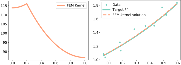
The image displays two side-by-side plots, likely from a scientific or engineering context, comparing a Finite Element Method (FEM) kernel function and its application in solving a target function. The left panel shows the kernel's profile, while the right panel compares the FEM-kernel solution against a target function and scattered data points.
### Components/Axes
**Left Plot:**
* **Type:** Line graph.
* **Legend:** Located in the top-right corner. Contains one entry: "FEM Kernel" represented by a solid orange line.
* **X-Axis:** Linear scale. Markers at 0.0, 0.2, 0.4, 0.6, 0.8, 1.0. No axis title.
* **Y-Axis:** Linear scale. Markers at 90, 95, 100, 105, 110. No axis title.
**Right Plot:**
* **Type:** Scatter plot with overlaid lines.
* **Legend:** Located in the top-left corner. Contains three entries:
1. "Data" - Teal-colored circles.
2. "Target f*" - Solid teal line.
3. "FEM-kernel solution" - Dashed orange line.
* **X-Axis:** Linear scale. Markers at 0.1, 0.2, 0.3, 0.4, 0.5, 0.6. No axis title.
* **Y-Axis:** Linear scale. Markers at 1.0, 1.2, 1.4, 1.6, 1.8. No axis title.
### Detailed Analysis
**Left Plot (FEM Kernel Profile):**
* **Trend Verification:** The orange "FEM Kernel" line begins at a high value, rises to a sharp peak, and then decays monotonically.
* **Data Points (Approximate):**
* At x = 0.0, y ≈ 113.
* The line rises to a peak at approximately x = 0.2, where y ≈ 116.
* After the peak, the line slopes downward. At x = 0.4, y ≈ 103.
* At x = 0.6, y ≈ 95.
* At x = 0.8, y ≈ 90.
* The line ends at x = 1.0, y ≈ 87.
**Right Plot (Solution Comparison):**
* **Trend Verification:** Both the "Target f*" (teal solid line) and "FEM-kernel solution" (orange dashed line) show a clear, consistent upward (positive) slope. The scattered "Data" points are distributed around these lines.
* **Data Series & Points (Approximate):**
* **Target f* (Teal Line):** A smooth, slightly concave-up curve. Starts near (0.07, 1.05) and ends near (0.60, 1.80).
* **FEM-kernel solution (Orange Dashed Line):** Closely follows the teal "Target f*" line, indicating a good fit. It is nearly indistinguishable from the target line across the plotted range.
* **Data (Teal Circles):** Approximately 15-20 scattered points. They follow the general upward trend but exhibit noise/scatter. For example:
* A cluster near x=0.1, y≈1.05-1.10.
* A point near x=0.2, y≈1.25.
* A point near x=0.3, y≈1.45.
* A point near x=0.5, y≈1.75.
* The scatter appears roughly symmetric around the trend lines.
### Key Observations
1. **Kernel Shape:** The FEM Kernel (left plot) is not a simple Gaussian; it has a distinct asymmetric peak near x=0.2 followed by a long tail.
2. **Solution Accuracy:** The "FEM-kernel solution" (orange dashed) provides an excellent approximation to the "Target f*" (teal solid), as their lines overlap almost perfectly in the right plot.
3. **Data Scatter:** The "Data" points in the right plot show moderate variance around the true/target function, suggesting the presence of noise in the observations that the FEM-kernel method is fitting.
4. **Spatial Relationship:** The two plots are presented together to first define the tool (the kernel) and then demonstrate its effectiveness in a reconstruction or regression task.
### Interpretation
This figure demonstrates the application of a specific Finite Element Method kernel for function approximation or solving an inverse problem.
* **What the data suggests:** The left plot characterizes the kernel's influence function, showing it has a localized peak, meaning it gives the most weight to data points near x=0.2. The right plot validates the method: despite noisy data, the FEM-kernel solution successfully recovers the underlying smooth target function `f*`.
* **How elements relate:** The kernel defined on the left is the fundamental building block used to generate the solution on the right. The close match between the orange dashed and teal solid lines indicates the chosen kernel and method are well-suited for this particular target function.
* **Notable patterns/anomalies:** The primary observation is the high fidelity of the reconstruction. The scatter in the data points is a normal feature of such problems, and the method's ability to ignore this noise and capture the trend is a sign of robustness. The lack of axis titles is a minor omission for a technical document, requiring the reader to infer the variables (likely a spatial or temporal coordinate on the x-axis and a function value or coefficient on the y-axis).