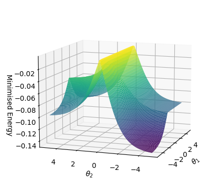
## 3D Surface Plot: Minimised Energy vs. θ1 and θ2 ### Overview The image is a 3D surface plot visualizing the relationship between "Minimised Energy" and two variables, θ1 and θ2. The surface is colored to represent the energy levels, with lower energy values appearing in purple/blue and higher energy values in yellow/green. The plot shows a complex energy landscape with a minimum point and varying degrees of curvature. ### Components/Axes * **X-axis:** θ1, ranging from approximately -5 to 5. Axis markers are present at -4, -2, 0, 2, and 4. * **Y-axis:** θ2, ranging from approximately -5 to 5. Axis markers are present at -4, -2, 0, 2, and 4. * **Z-axis:** Minimised Energy, ranging from -0.14 to -0.02. Axis markers are present at -0.14, -0.12, -0.10, -0.08, -0.06, -0.04, and -0.02. ### Detailed Analysis The surface plot shows the following trends: * **General Shape:** The surface has a valley-like structure, indicating a region of lower energy. There is a clear minimum point in this valley. * **Energy Minimum:** The minimum energy value appears to be around -0.14, located near θ1 = 0 and θ2 = 0. * **Energy Peaks:** There are two peaks in the energy surface, one on each side of the valley along the θ2 axis. The peaks reach a maximum energy of approximately -0.02. * **Symmetry:** The plot appears to be roughly symmetrical with respect to the θ1 axis. ### Key Observations * The plot clearly shows a minimum energy configuration for the system being modeled. * The energy landscape is not uniform, with significant variations depending on the values of θ1 and θ2. * The presence of peaks suggests that there are other, less stable, configurations. ### Interpretation The 3D surface plot visualizes an energy landscape, likely representing a system where the energy is dependent on two parameters, θ1 and θ2. The plot demonstrates that there is a specific combination of θ1 and θ2 that minimizes the energy of the system. The shape of the surface indicates the sensitivity of the energy to changes in these parameters. The presence of peaks suggests that there may be other local minima or saddle points in the energy landscape, which could correspond to metastable states of the system. The plot is useful for understanding the stability and behavior of the system as a function of θ1 and θ2.