## [Chart Type]: Dual Line Plots of Convex Function Cross-Sections
### Overview
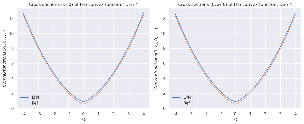
The image displays two side-by-side line charts, each plotting a cross-section of a convex function in 4 dimensions. The charts compare two data series labeled "LPN" and "Ref" across a symmetric domain. The visual style is a standard scientific plot with a light grid background.
### Components/Axes
**Titles:**
- Left Plot: `Cross sections (x₁,0) of the convex function, Dim 4`
- Right Plot: `Cross sections (0, x₂,0) of the convex function, Dim 4`
**Axes:**
- **X-axis (Left Plot):** Labeled `x₁`. Scale ranges from -4 to 4, with major tick marks at integer intervals (-4, -3, -2, -1, 0, 1, 2, 3, 4).
- **X-axis (Right Plot):** Labeled `x₂`. Scale and ticks are identical to the left plot.
- **Y-axis (Both Plots):** Labeled `Convexfunctions(x₁, 0, ...)` (left) and `Convexfunctions(0, x₂, 0, ...)` (right). Scale ranges from 0 to 12, with major tick marks at intervals of 2 (0, 2, 4, 6, 8, 10, 12).
**Legend (Bottom-Left of each plot):**
- **LPN:** Represented by a solid blue line.
- **Ref:** Represented by a dashed orange line.
### Detailed Analysis
**Data Series Trends:**
Both plots show two U-shaped, symmetric curves centered at x=0, characteristic of a convex function.
1. **Left Plot (x₁ cross-section):**
- **LPN (Blue, Solid):** The curve has its minimum at approximately (0, 1.0). It rises symmetrically to a value of approximately 12.5 at x₁ = -4 and x₁ = 4.
- **Ref (Orange, Dashed):** The curve has its minimum at approximately (0, 0.5). It rises symmetrically to a value of approximately 12.5 at x₁ = -4 and x₁ = 4.
- **Relationship:** The LPN curve is consistently above the Ref curve across the entire domain. The vertical offset is greatest at the minimum (≈0.5 units) and diminishes to near zero at the extremes (x=±4).
2. **Right Plot (x₂ cross-section):**
- The trends, shapes, and numerical values are visually identical to the left plot. The LPN curve (min ≈1.0) sits above the Ref curve (min ≈0.5), with both converging at the boundaries (x₂=±4, y≈12.5).
**Spatial Grounding & Value Confirmation:**
- The legend is positioned in the bottom-left corner of each plot's axes area.
- The blue solid line (LPN) is the upper curve in both plots.
- The orange dashed line (Ref) is the lower curve in both plots.
- The minimum point for both series occurs precisely at x=0 on the horizontal axis.
### Key Observations
1. **Systematic Offset:** There is a consistent, positive vertical offset between the LPN approximation and the Reference function across both cross-sections.
2. **Shape Preservation:** Despite the offset, the LPN curve perfectly preserves the convex, symmetric shape of the Reference function.
3. **Convergence at Extremes:** The two curves converge as the absolute value of the input variable increases, suggesting the approximation error is largest near the function's minimum.
4. **Identical Cross-Sections:** The behavior of the function is identical along the x₁ and x₂ axes (with other variables fixed at 0), indicating symmetry in the function's definition with respect to these variables.
### Interpretation
This figure demonstrates the performance of an approximation method (LPN) against a reference function (Ref) for a convex function in 4-dimensional space. The key takeaway is that the LPN method successfully captures the fundamental convex geometry and symmetry of the target function. However, it introduces a systematic bias, overestimating the function's value, particularly near its global minimum. The error is not uniform; it is most pronounced at the center of the domain and becomes negligible at the boundaries of the plotted region. This pattern suggests the approximation may be less reliable for tasks requiring high precision near the function's minimum, such as optimization, but is structurally sound for understanding the function's overall landscape. The identical nature of the two cross-sections implies the underlying function treats the first two dimensions equivalently.